Editor’s note: Don Minchow is president of Inquire Market Research, Inc., Santa Ana, Calif.
Some of you are old enough to remember when Bill Cosby was a stand-up comedian and his routines could be heard on record albums. (For those of you born after the introduction of CDs, a record album is a large vinyl disk that was played on something called a turntable.) One of his famous bits involved wondering how Noah must have felt when instructed by God to build an ark. It went something like this:
God: “Noah, I want you to build an ark that is 300 cubits by 500 cubits.”
Noah: “Right. What’s a cubit?”
I was reminded of this interchange when a client requested a proposal for a research study to demonstrate the effects of various lens coatings on visual acuity. Of course, his first question was, “How large a sample do I need?” From there, our conversations went something like this:
Me: “How confident do you want to be of your research findings?”
(Unlike some of my clients, this on had an answer.)
Client: “Quote me at 99 percent, 95 percent, and 90 percent confidence levels.”
Me: “That’s a great start. How much of a difference do you expect to see between the mean readings for each coating?”
Client: “Not sure, why don’t you figure a range from .02 to .1, in increments of 0.2.”
Me: “Now we’re cooking; we’ve got the confidence levels and the differences in the means. All we need now is the standard deviation. What do you want to use?”
It was at this point that I flashed back to Cosby’s routine. My client got the look of a deer caught in the headlights of an oncoming car, and he mumbled something to the effect of, “Right. What’s a standard deviation? And more importantly, how should I know what it is for this study?”
Me: “Well, in simple terms, the standard deviation is the measure of dispersion.”
Client: “Right. What’s dispersion?”
I don’t know what I was thinking. This explanation didn’t mean anything to me the first time I heard it from a statistics professor. What made me think it was going to be any more meaningful for my client? So I backed off a little, and gave him an explanation.
Me: “Let me give you an example: What is the average of two, six, and 10?”
Client: “It’s six.”
Me: “Right. Now, what’s the average of five, six and seven?”
Client: “That’s six also.”
Me: “Right. The average of both series is six, but you can see that one group of numbers stretches from two to 10 and the other is limited to a much smaller range, from five to seven. So, in this case, the first range of numbers, from two to 10, is widely dispersed, and has a standard deviation of 3.3. The second range is narrowly dispersed, and has a much smaller standard deviation, it’s only 0.8. The same principle holds true for much larger samples. If each of the numbers in a series is close to the overall average, the standard deviation is small. If the numbers are all over the map, the sample has a large standard deviation.”
Client: “That makes sense. But how am I supposed to know what it will be for this study?”
Me: “That’s a tough one. Usually we rely on findings from similar studies. Have you ever done this type of study before?”
Client: “Well no, but we do have the raw data from a number of exams that have been done by one of our customers over the past year.”
Me: “Perfect! Get me the raw data and we’ll enter it into the computer. If we can assume the population we’ll be testing in this new study is similar to the one your historic data is based on, then it will work in our formula.”
Crunching the numbers
Fast-forward three weeks. We have received the exam sheets, entered the data into the computer, calculated the mean and standard deviation. We have concluded from this pilot study that the standard deviation for this sample population is .33. Now it’s time to give the client some insights into the sample size necessary to provide him the results he needs.
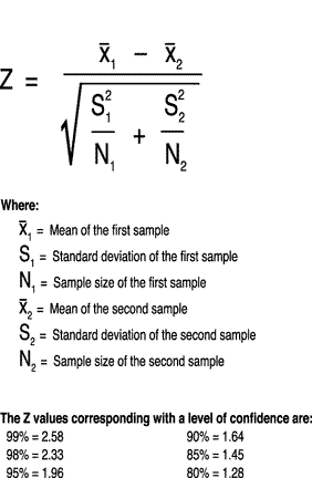
All I can say is, thank God for automated spreadsheets. We started the process by using the formula for Z tests.
 |
We selected a range of differences for the means, and we chose a range and interval of sample sizes to calculate the Z values. Once the values were calculated, they were examined for reasonableness, and to see where we were for sample size. The table we generated is shown below.
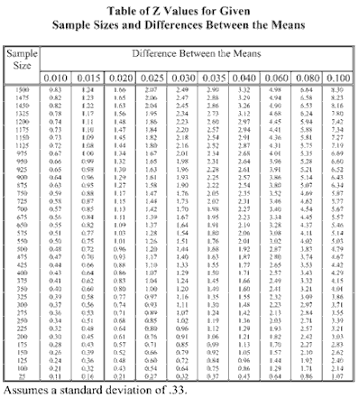 |
While this is a good first step, and it is possible to search the table and find the appropriate Z value, this table is difficult to read. So I created a second table (below) to interpret the results of the first. Using the “@IF” function, I tested each value to determine the confidence level for the Z value in the cell. Redundant responses have been eliminated as you read across the table from left to right, just to make the table easier to read.
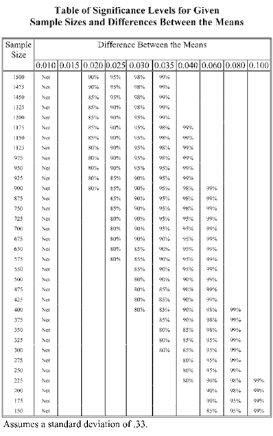 |
The results were very readable, and the table would have served our purposes nicely. However, never one to leave well enough alone, I decided to graph the findings so we’d have a simple exhibit to use as a quick reference the next time we encountered a study with similar variables.
The graph plots the sample size for each of the Z values associated with the levels of confidence. For example, the top line on the graph is for the Z value 2.58, and the 99 percent confidence level. If we want to be 99 percent confident that a difference in the means of 0.025 represents a real difference in lens performance and not a random occurrence, we’ll need to test a minimum of 2,320 subjects.
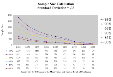 |
In order to plot these figures, we have to solve the above formula for N. In other words, we are solving for the sample size that represents the threshold value, or the sample size for a given standard deviation and Z value that marks the end of one level of confidence and the beginning of another. In the above example, the sample size of 2,320 is the threshold, or the lowest sample size, where a difference of 0.025 in the means of two samples, and a standard deviation of .33, is significant at the 99 percent level of confidence.
Since we’re assuming the sample size and standard deviation for each lens tested will be the same, the formula is:
Sample Size = 2(S2 * Z2)/∆x
Where:
S is the assumed standard deviation for both samples;
Z is the Z value;
∆x is the difference between the mean readings for each lens coating.
The resulting graph is shown on the opposite page.
Not rocket science
Obviously, this is not rocket science. And there are probably statisticians among you who will find something about this approach to criticize. But I find that my clients are less concerned about the subtle distinctions to be made between various statistical approaches and are more interested in answering their business questions. The preceding exercise demonstrates a real-world approach to tackling one of the issues that frequently results in anxiety and procrastination.
