
Editor's note: Albert Madansky is H.G.B. Alexander Professor Emeritus of Business Administration, Chicago Booth School of Business, University of Chicago. He is also vice president, The Analytical Group Inc., a Scottsdale. Ariz., research firm.
The widely used Net Promoter Score (NPS) was introduced in Reichheld (2003) and is calculated based on responses to a single question: “How likely is it that you would recommend our company/product/service to a friend or colleague?” where the response is given based on a 0 to 10 scale. Respondents with scores of 9 or 10 are called Promoters, those with scores of 6 or below are called Detractors and those with scores of 7 or 8 are called Passives. The NPS is defined as 100 times the difference between the fraction of Promoters and the fraction of Detractors in the sample. There are a number of contexts in which researchers are interested in comparing NPSs to see if they are significantly different. In this article I will set forth the basic principles for performing such statistical comparisons.
Multinomial distribution basics
Consider a multinomial population with k categories whose corresponding means are θ1, …,θk. Assume that we have a random sample of n observations from this population, with observed category proportions p1, p2, …, pk, where
 Since the sum of the p’s is 1, the p’s are negatively correlated (if one of the pi is large the other pjs will perforce be small).
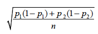
Suppose we wish to test the hypothesis that θ1 = θ1, based on the statistic p1 – p2. As shown by Wilks (1940), the standard deviation of the statistic p1 – p2 is
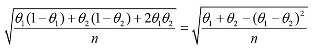 Since the θ’s are unknown, we estimate them by their sample estimates and use as an estimate of the standard deviation of p1 – p2 the quantity
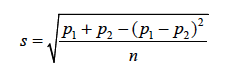 A common error made by those comparing two percentages from a multinomial distribution is to treat them as independent. In doing so they erroneously calculate the estimated standard deviation as
 thereby underestimating the standard deviation and hence declaring non-significant differences as significant.
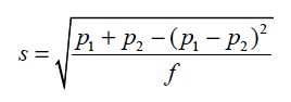
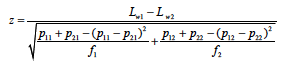
To apply this to NPS we let k=3, with subscript 1 representing Promoters, subscript 2 representing Detractors and subscript 3 representing Passives. Then (except for a factor of 100) p1 – p2 is the NPS and s given above is an estimate of the standard deviation of the NPS. If therefore one wanted to compare two NPSs, say L1 and L2, computed from two independent samples of sizes n1 and n2, respectively, one would calculate the z-statistic
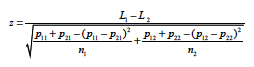
where p11 and p12 are the Promoter fractions and p21 and p22 are the Detractor fractions in the respective independent samples.
Some researchers cleverly code the Promoters as 1, the Detractors as -1 and the Passives as 0, calculate L1 and L2 as the averages of these coded data and then use the two-sample t-test to test the significance of the difference. This leads to a minor error, which can be seen from the following analysis. One of the computations in facilitating the t-test is the calculation of the sample variance of La. Let the scores of the na respondents be denoted as  . Then the sample variance for sample a (a = 1, 2) is calculated as
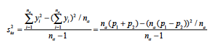
and the squared standard error of La is calculated as
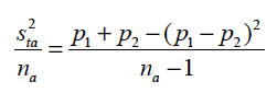 instead of as
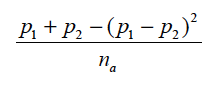 While this error is negligible for large samples, it can make a difference for small samples.
Weighting
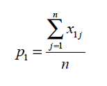
To develop the comparable procedure when the data are weighted, assume that the j-th member of the sample is given weight wj, j=1, … , n, We represent the data as a collection of nk 1’s and 0’s, with xij being a 1 if respondent j responded positively to category I and xij =0 otherwise. Then for example p1 can be written as
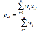
 The weighted pw1 can be expressed as
 The determination of the standard deviation of the statistic pw1 – pw2 is based on the following:
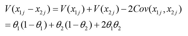
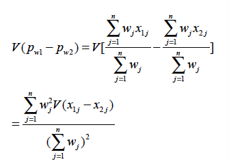 But
But
 So
So
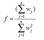
 where f is the effective sample size, called the “design effect” by Kish (1965, Section 8.2, p. 258).
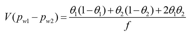
 Since the θ’s are unknown, we estimate them by their sample estimate and use as an estimate of the standard deviation of pw1 – pw2 the quantity
 If therefore one wanted to compare two NPSs, say Lw1 and Lw2, computed from weighted data from two independent samples of effective sample sizes f1 and f2, respectively, one would calculate the z-statistic
More complex comparisons
Market researchers may sometimes compare NPSs from samples that may not be independent. One might ask a respondent the basic rating question about two different products. To complicate matters, some respondents may only rate one of the products rather than both. Obviously the ratings are correlated (because we may have the same respondent rating both products), so that the NPSs are correlated. To further complicate matters, the responses to each of the products rated by those respondents who rated both products may be assigned different weights.
Another scenario is one where the basic rating question is asked about a product and then the sample is split into (not necessarily separate) subgroups and one wants to know if the average NPSs are different for these subgroups. For example, we may ask whether the average NPS for users of Product A is different from that of Product B, where some of the respondents are users of both products. Again, to further complicate matters, the respondents may be weighted differently for product A and for Product B. The Analytical Group has developed appropriate statistical procedures to handle all these complexities, which have been incorporated into the newest version of WinCross.