Inside the black box
Editor's note: Based in San Antonio, Texas, Alexander C. Larson and Basile Goungetas are economists in the consumer wireline and direct marketing department at AT&T.
The concept of Net Promoter Score (NPS) has become a popular method of satisfaction and loyalty measurement at most large and medium-sized firms in American industry. Essentially, NPS is a relationship measure that gauges a customer’s willingness to recommend a given firm. It has its genesis in the original article by Frederick Reichheld (“The one number you need to grow,” Harvard Business Review, December 2003). The resulting implementation of NPS is relatively simple: a survey is administered to Firm X’s customers, containing the following question: How likely is it you would recommend Firm X? The question is administered on an 11-point scale, with each survey respondent answering the question with a score of from 0 to 10. Those who respond with a value of 0 through 6 are designated as Detractors; those responding with a 7 or an 8 are designated as Passives; and those responding with a 9 or a 10 are Promoters. From the survey data collected, NPS is a simple calculation: the percent of promoters minus the percent of detractors.
That’s fine as far as it goes; but what if Firm X wants to go further? Suppose that the executives and line managers of Firm X want to use customer experience measurement results to improve business outcomes? Suppose they want to know what actually determines a satisfaction measurement like NPS, so that they can take steps to improve it? This is where a driver analysis comes in. A driver analysis tells the business executive which controllable factors have an effect on NPS and how much of an impact they have. It allows the executive to take steps to improve NPS and tells him or her how much improvement to expect from changes in a given driver. In other words, driver analysis enables the decision-maker to play what-if games to see how changing a measurable driver of NPS can improve results (e.g., a reduction of Detractors, an increase in Promoters, etc.).
But exactly how is a driver analysis conducted for a satisfaction measure like NPS? A statistical model is constructed to compute the probability that a survey respondent selects a given value of the 11-point scale, such as a 0, a 6 or a 10, etc. This lets the analyst compute and simulate the probabilities of Promoters, Detractors and Passives (and hence NPS) under a variety of scenarios. The model could also have just three categories (Promoters, Passives and Detractors) in lieu of all 11 points of the scale, though the full scale offers more detail.
This is where applied econometrics comes in. The econometrician has tools that can be used to conduct a driver analysis for NPS. The right tool will depend, in part, on how the data are processed and presented to the analyst. Two primary methods can be used for NPS driver analysis: the ordered logit model and the grouped logit model. Which model is the right tool for the job?
Ordered logit. If the raw data contains the responses to the Net Promoter question (How likely is it you would recommend Firm X?) at the individual survey respondent level (with numbers from 0 to 10), then the ordered logit model is appropriate. The ordered probit model is also appropriate with this kind of data.
Grouped logit. If the data have been aggregated across individual survey respondents who reside in, for example, geographic sales regions, then the grouped logit model is appropriate. For example, a research manager may produce a report that says the West Sales Region has 40 percent Promoters, 30 percent Passives and 30 percent Detractors, yielding a NPS of 10 percent. This is the kind of data for which grouped logit would be used, assuming you have a large number of sales regions.
The right method depends on the question at hand and the data available to the analyst conducting the driver analysis.
Ordered logit
The overarching reason for conducting a driver analysis is to parse NPS with respect to the various factors that determine it. To accomplish this, the analyst uses statistical analysis to develop a mathematical formula or model yielding NPS as a function of the factors or drivers that determine it. With such a model in hand, the analyst can run simulations to determine the practical impact that a given factor has on NPS.
If the analyst has raw data on the survey responses to the willingness-to-recommend question, he or she will have a response rating (a number from 0 to 10) for each survey respondent. This is the data to model on the left-hand side of the model equation. Presumably, there will also be data on potential drivers at the individual survey respondent level; these will constitute the explanatory variables, or drivers, on the right-hand side of the model equation. If this is so, then the analyst can model NPS using ordered logit. The raw NPS number itself is not actually modeled; the probabilities of each response (0 to 10) or each of three categories (Promoters, Passives and Detractors) are modeled. This enables driver analysis of NPS.
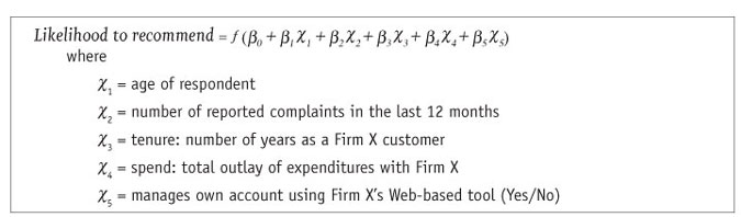
Below is a simplified example of the driver equation, using individual-level survey data for the question (How likely is it you would recommend Firm X?).

The ordered logit model is a method for modeling qualitative and limited dependent variables, such as the data from a NPS survey. Thus, one can use it to model a dependent variable whose values are confined to just the integer values 0 through 10, and that exhibits ordering. If a variable is ordinal, its values can meaningfully be ranked from low to high. The ordered logit model can simulate the probability of each willingness-to-recommend rating (0 to 10) each survey respondent could have selected, with all such probabilities summing to 100 percent. The analyst can then simulate the probability that a given survey respondent would have been a Net Promoter. How? The ordered logit model can predict the probability of selecting a 9 or higher (a Promoter) and the probability of selecting a 6 or less (a Detractor). For each respondent, the simple subtraction of Detractor probability from Promoter probability yields that survey respondent’s estimated probability of being a Net Promoter. For the sample, the simple mean of these probabilities across all respondents is computed to yield an overall NPS.
Unfortunately, the ordered logit model is not the easiest model to implement in practice; the function ƒ shown above is nonlinear. Unlike other types of modeling techniques, there are two ways to parameterize the ordered logit model, not a single way, as is true of many other workhorse models researchers use. The way a model is parameterized involves the formulae that a statistical package will use behind the scenes to estimate that model. Thus, for a given statistical computing package, the challenge for the practitioner is to know how that package parameterizes the ordered logit – and this is just a fancy way of saying the analyst must be certain what formulae his package of choice uses when estimating the ordered logit model. If there are two ways this model can be parameterized, then which way does your package use? Without this knowledge, it is possible to estimate the ordered logit model but impossible to simulate it reliably and hence do the driver analysis – and the driver analysis is the name of the game.
So, how do real applied econometricians do this? The formula that underlies the ordered logit model (and many, many others) is its likelihood function. Usually, if an econometrician wishes to confirm which formulae a statistical computing package will use to estimate a given model, he or she will remove all doubt by inputting the likelihood function directly, using a statistical procedure that enables this. In SAS, PROC NLP or PROC NLMIXED can be used, or programs such as TSP or Gauss, as but four examples. The analyst selects the model of interest (such as ordered logit); inputs the likelihood function (including all parameters required for the driver analysis); and then maximizes the likelihood function for the sample of survey data collected. This allows a manual estimation of the model of interest, independent of the canned programming available (but equivalent). All formulae are set by the analyst and there is no doubt as to which version of the desired model has been estimated. If the manual estimation matches the canned program, you know what your stat package is doing.
Thus, when estimating the ordered logit model to analyze NPS, some econometricians will eschew the standard canned computing routine (such as PROC LOGISTIC in SAS) and, essentially, build their own. This approach allows more flexible nonlinear models that canned programs cannot produce and ensures that the NPS driver equation will be simulated correctly. We have seen well-established market research vendors stumble when trying to simulate the impact of drivers on measures similar to NPS; ordered logit can be treacherous ground indeed. It is not a good candidate for a “plug and chug” approach, using a statistical package’s canned computing routines.
So, suppose you are tasked with a driver analysis of NPS. You decide to use the ordered logit model. If you don’t know which parameterization of the likelihood function your statistical package uses “inside the black box” to estimate this model, don’t guess and don’t take it on faith. Why not just input its likelihood function yourself? This likelihood function and the way it is parameterized is available in standard textbooks. That would allay all fears of a “black box” outcome, wouldn’t it? The authors use a well-known source as a guide for programming the ordered logit likelihood function in SAS: J. Scott Long’s book Regression Models for Categorical and Limited Dependent Variables. The ordered logit can be estimated this way and this is the method the authors prefer but it is a bit trickier than estimating other models manually. Why? It requires the user to be comfortable with the concept of maximum likelihood estimation and to program the formulas used for interpreting, predicting or simulating the model after it is estimated. It also requires a setup unlike similar models.
Thus, the ordered logit model is not a model for beginners. But once a good template for the programming code in a statistical computing package is available, it is not a daunting model for driver analysis. The trick is to set up a correct template program in a package such as SAS or TSP and use that template for quick and reliable estimation. Even seasoned professionals use templates to save time, eliminate tedious code-writing and lower the likelihood of human error. (Sample SAS code that can be used to estimate ordered logit and grouped logit models is available from the authors on request.)
This approach offers several advantages, from a technical and statistical perspective, but perhaps the biggest advantage is the peace of mind the analyst enjoys by knowing that he or she has a great deal of control over the analysis; the quirks or uncertainties of various canned computing routines become a moot issue.
Grouped logit
As we indicated earlier, if you are starting with data that has been aggregated across survey respondents in some way, then the grouped logit model could be appropriate, depending on how much data you have. Instead of having observations from a single individual, you have observations on Promoters, Passives and Detractors aggregated to a higher level. You are no longer modeling NPS for individuals; you are modeling NPS for groupings of people and the data you have are the aggregate percents of Promoters, Passives and Detractors for the groupings (plus the grouped data on the drivers).
But how would a situation like this come about? Consider the following scenario: you are all set to do a driver analysis of NPS using data at the individual survey respondent level. You have a great deal of survey data to work with. And at that point your client tells you that he wonders what impact the number of salespeople has on NPS. You notice that you don’t have data on number of salespeople for individual survey respondents but you do have that data for each of 300 designated company sales regions. The client then tells you he wants to know if another 10 variables also affect NPS, such as: number of stores, amount of advertising in local newspapers, etc. You face the same problem: there are data on his suggested variables aggregated up to the level of the 300 standard sales regions but – you guessed it – not for your individual survey respondents. The client’s data come from standard company reports and even if you wanted to, you could not ask anyone about it in a survey.
So what do you do? You analyze NPS using grouped logit. Here are some steps to follow for a workflow:
1. Prepare the data set for the grouped logit model. In this example, it requires the analyst to:
a. Compile the data his client has provided from company reports.
b. Compute the percents (aggregated) for each value of the rating scale (0 through 10) for each of the 300 sales regions. You may also use just three categories for Promoters, Passives and Detractors, though the full scale is more flexible.
c. Aggregate any applicable survey data up the sales region level.
2. Estimate a grouped logit model. This can be done two ways:
a. Build your own. Use the same method described above: Feed the likelihood function for the grouped logit into a computing routine that allows you to estimate this model manually, such as PROC NLMIXED or PROC NLP in SAS. This is the approach the authors prefer, because it makes simulation of the model a bit easier and removes all doubt as to which model has been estimated.
b. Canned computing routine. Use your stat program’s canned computing routine for grouped logit, such as PROC LOGISTIC or PROC GENMOD in SAS – but as always, be certain you know how the model is being computed inside the black box so that you can conduct driver analysis.
A simulator for driver analysis
After you have estimated the model, the estimated model parameters are used to create a simulator for driver analysis of NPS. The simulator enables the analyst to play what-if games and see how the probabilities of Promoters and Detractors (and hence NPS) change as drivers are altered or tinkered with. It computes the probabilities of Promoters, Detractors and Passives for given values of the driver variables. Thus, it enables the user to see how NPS changes as the values of drivers change. Simulators are usually constructed using your own statistical package or by building an Excel-based simulator. This is the main tool for driver analysis. The simulator can be handed off to line managers so they can see the NPS impact of various scenarios.
A fair question is: Why does this driver analysis have to be so complex? Why can’t a much simpler method be used? A research manager may complain that he doesn’t have Nobel Prize-winning econometrician Daniel McFadden or professors Ken Train or Moshe Ben-Akiva sitting in a cube, ready to analyze NPS drivers.
For instance, how about the multinomial logit (MNL) model? The MNL is ubiquitous in market research – why not just use that in lieu of ordered logit? It is much simpler to use in practice. If there is ordering in the data, as is true with the ratings data used to compute NPS, then ordered logit probably trumps the MNL model. It is a more efficient estimator in general, meaning the estimates you will get from using it will have a smaller variance and be more precise. Nonetheless, it may still be useful to estimate a model with ordinal outcomes using MNL (which is designed for nominal outcomes) – it depends. Using MNL is not a silly thing to do in this instance but ordered logit would likely be better.
Similarly, for the grouped aggregated data, why not just compute NPS for each group and model it directly using ordinary least squares (OLS)? What’s wrong with that? First, NPS is bounded by -1 at the low end and 1 at the high end. OLS can yield NPS that can go outside the bounds of -1 to 1 and that would make no sense. Second, OLS cannot tell you how probabilities of Promoters, Passives and Detractors change as drivers change. Grouped logit can – that’s the level of detail and sophistication you want. Third, you can reasonably expect the effects of the drivers to have diminishing returns as you approach the NPS bounds of -1 or 1. A linear model cannot handle this but logit models can – they have S-shaped relationships between drivers and probabilities for Promoters, Passives and Detractors.
And why can’t an analyst just use OLS in lieu of ordered logit? In this case, the left-hand-side variable is just numbers from 0 through 10 – why ordered logit in lieu of the much easier OLS? OLS is inappropriate to apply to the individual survey respondent data, largely for the same reasons cited above. And the intervals between adjacent values or categories of an ordinal variable (defined by “cutpoints” or “thresholds”) are not necessarily uniform but OLS assumes they are. Logit models handle this, OLS does not.
Does not tell the whole story
The concept of net promoter score is a popular and pervasive method of satisfaction measurement at most large and medium-sized firms in American industry. However, the NPS itself does not tell the whole story. Line managers want to know what determinants of NPS will move the needle. This is where a driver analysis of NPS comes in. Driver analysis can answer common questions raised about NPS: What attributes of a sales operation affect NPS the most or the least? How can I improve NPS?
If driver analysis of NPS is important, then it is important enough to do correctly. Though ordered logit and grouped logit are not the only tools in the shed, they are primary workhorse methods for NPS driver analysis. These methods are not for neophytes and require some statistical maturity (i.e., a knowledge of how to specify and estimate the likelihood functions for ordered or grouped logit and then simulate the results). If you commission a NPS driver analysis from an outside research vendor, don’t be shy about asking which method they will use. If they can’t defend their planned method, don’t be afraid to pick another vendor. And do some sanity checks on the simulator after you receive it – this is where the pitfalls of ordered logit will affect the final delivered product the most.