

A pricing method for two-attribute trade-offs
Editor's note: Westley Ritz is vice president of analytics at TRC Insights, with 20 years of experience in consumer insights and advanced analytics and pricing research. He holds an M.S. in statistics from Temple University and a B.S. in statistics and economics from the University of Michigan. Find Ritz on LinkedIn.
A decade ago in this magazine, Rajan Sambandam laid out a framework for practical pricing research.1 The framework matches the right method to the product development stage. Early-stage with features still being defined calls for stated purchase intent methods like the Van Westendorp price sensitivity meter, split-cell monadic or sequential Gabor-Granger. Mid-to-late-stage with firmed-up features and competitive context calls for conjoint analysis, typically choice-based. But a class of pricing problems shows up in client briefs that doesn't fit cleanly in either bucket. The single-attribute methods are too narrow. A full conjoint is too broad. The problem sits in between.
Consider a healthcare consumer choosing between a virtual doctor visit at a particular co-pay price and a 1-day wait for the appointment or an in-person visit at a different price and a 7-day wait. The decision turns on two numbers (co-pay price and wait time) and both have to vary to measure the trade-off. Single-attribute methods don't apply because wait time is material to the decision and can't be held fixed. A full conjoint design works but it's more design and modeling effort than a two-attribute problem requires. The deliverable the client typically wants is the take rate at each (price, wait) combination, with the revenue-maximizing price easily derived.
The same pattern shows up in other industries. Streaming subscribers weighing price against ad load. Telecom subscribers weighing price against data allowance. Buy-now-pay-later customers weighing interest rate against repayment term. Insurance buyers weighing premium against deductible. In each case, the problem involves two quantitative attributes that both have to vary in order to measure the price-service trade-off.
Two-dimensional Gabor-Granger
An adaptation of the Gabor-Granger method handles this type of problem. We call it 2D Gabor-Granger. Classical Gabor-Granger asks a respondent a sequence of purchase-intent questions across a price ladder, adapting upward when the respondent says yes and downward when they say no, until the maximum acceptable price is found.2 2D Gabor-Granger does the same thing in two dimensions at once. Instead of a price ladder, the method uses a grid of (price, second-attribute) combinations. Each answer classifies a region of the grid rather than a single cell.
The practitioner defines the grid. For a healthcare study, that might be a 5x5 grid of co-pay prices (e.g., $10, $20, $30, $40, $50) and wait times (e.g., same-day, 1-day, 3-day, 7-day, 10-day). Each cell is one possible (price, wait) combination. The respondent answers a sequence of accept/reject questions, with each next question chosen adaptively based on prior answers. The result is each cell classified as acceptable or unacceptable, in the original attribute units (dollars and days). Some classifications come from direct answers and the rest fill in by dominance from related answers.
Grid design is a practitioner decision. The grid doesn't have to be square and levels within an attribute don't have to be evenly spaced. Both axes should reflect real decision breakpoints: prices that the client is genuinely weighing and second-attribute levels that match how customers actually think about the choice (same-day, next-day, this-week and so on for wait time). Price levels typically cover the testable range plus a buffer at each end in case relevant prices fall outside the initial range. The dominance logic only needs each attribute to have a consistent preference direction (lower price always preferred, shorter wait always preferred).
The efficiency comes from dominance. If a respondent would book the virtual visit at $40 co-pay with a 3-day wait, they would also book it at any lower price with the same or shorter wait and at the same price with a shorter wait. Those cells fill in without being asked. The logic runs the other direction too: if the respondent rejects a cell, any cell that's worse on both attributes is also rejected. The adaptive method asks questions only in the unanswered region of the grid and each answer fills in more of it.
Walking through the task
Figure 1 shows a 3x3 example: how one respondent's answers fill in all nine cells across four tasks (actual number of tasks will vary by respondent). Columns represent price ($, $$, $$$) and rows represent wait time (Short, Medium, Long). Lower price and shorter wait are preferred, so the upper-left cell is best and the lower-right cell is worst. Each task is chosen to bisect the remaining unanswered region: the cell whose answer will split it most evenly.
The four tasks fill the full grid:
Task 1: Ask center cell ($$, Med). Respondent accepts. The asked cell plus three more (the top-left 2x2) fill in as accept by dominance. Five cells remain unanswered.
Task 2: Ask ($$$, Med). Respondent rejects. The asked cell plus one more fill in as reject by dominance. Three cells remain unanswered.
Task 3: Ask ($$$, Short). Respondent accepts. Only the asked cell fills in (no new dominance, because the cells it would dominate are already answered). Two cells remain unanswered.
Task 4: Ask ($, Long). Respondent rejects and dominance fills in the last unanswered cell. The grid is complete.
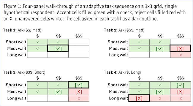
Reading the final state: At short waits for a virtual visit, the respondent will pay up to $$$. At medium waits, only up to $$. At long waits, they won't book at any tested price.
Task counts scale slowly with grid size. For a 4x4 grid, a typical respondent answers around six adaptive tasks before the grid is fully answered. For a 5x5, around eight tasks.
Deployment
The respondent task can be set up two ways. In monadic mode, each task presents a single offer and asks whether the respondent would purchase at that combination. This is the format familiar from classical Gabor-Granger and it suits new products without a natural competitive reference. In competitive mode, each task presents two offers: the test offer (which varies task to task per the adaptive logic) and a fixed reference offer (typically the in-market option or competitor). The respondent chooses one. This format puts the read in competitive context. The dominance logic is identical in both modes.
In competitive mode, a respondent might see:
A: In-person visit, $30 copay, 7-day wait. B: Virtual visit, $40 copay, 1-day wait. Which would you choose?
In monadic mode, the format simplifies to a single offer with an accept/reject response:
Would you book a virtual visit at $40 copay with a 1-day wait?
If intent is collected on a rating scale instead of binary accept/reject, dichotomize to top-box or top-two-box (treating the top one or two ratings as accept) before applying the dominance logic.
From task to deliverable
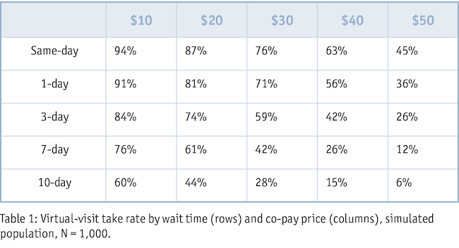
Each respondent's answers fill in the grid. Aggregating across respondents produces the standard pricing deliverables, extended into two dimensions. The illustrations in Table 1 come from a simulated healthcare pricing study of 1,000 respondents in competitive mode: a virtual visit at varying prices and wait times (as described previously), tested against a fixed in-person reference (in-person at $30 copay, 7-day wait). The numbers are illustrative of form, not findings about virtual healthcare.
The primary output is the take rate: the share of respondents who would choose the virtual visit at each (price, wait) combination, against the fixed in-person reference.
Reading across any row gives the demand curve at a fixed wait level. At same-day availability, take rate falls from 94% at $10 to 45% at $50. Reading down any column gives the response to wait time at a fixed price. At $30, take rate falls from 76% at same-day to 28% at 10-day. A single price ladder gives one demand curve at one fixed level of the other attribute. The grid gives five demand curves at once (one per wait level), plus the wait response at each price.
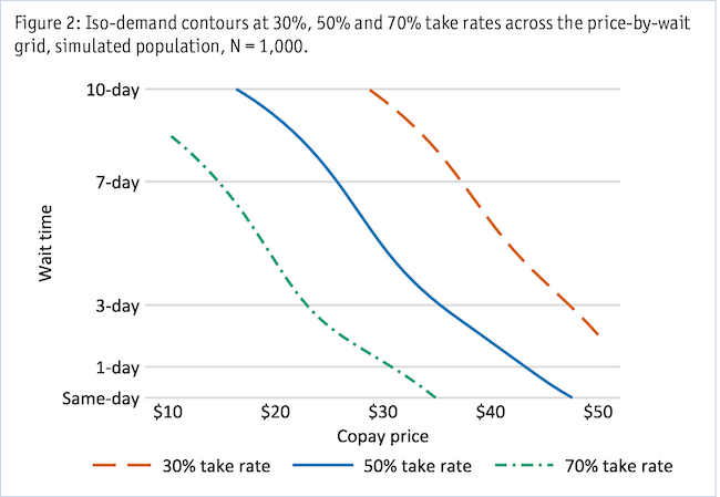
Figure 2 plots the same take rates as iso-demand contours, an alternative view of the demand surface.
Each contour traces the (price, wait) combinations that yield the same take rate. The 50% contour, for example, shows every combination that retains half the simulated population: higher prices at shorter waits, lower prices at longer waits. The contour view lays out the strategic options side by side at each target share, ready for comparison.
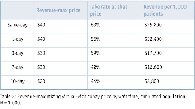
Multiplying take rate by price at each combination gives the revenue at each cell. Table 2 reports the revenue-maximizing price at each wait level among the tested prices, with the take rate and revenue per 1,000 patients at that price.
Same-day delivery produces the highest revenue but also requires the operational capacity to deliver same-day. Longer waits at lower prices produce less revenue per respondent but require less operational investment. The table quantifies that trade-off for that business decision.
Alongside the aggregate outputs, each respondent's threshold points are available as individual-level data. This supports subgroup analysis: median willingness to pay across wait levels by segment or demographic cuts. The simulation here splits the population between a convenience-oriented segment (n=400, willing to pay more to reduce wait time) and a price-sensitive segment (n=600). The convenience-oriented segment supports a $10 premium over the price-sensitive segment at the same-day, 1-day and 3-day waits, a $5 premium at seven days and no premium at 10 days. Cutting the results by segment lets the business see whether approaches such as tiered pricing or self-selection are worth pursuing.
Where 2D Gabor-Granger fits
The method to use depends on the problem. When one attribute is varying, classical Gabor-Granger or Van Westendorp may be the right tool. When two quantitative attributes vary and both drive the decision, 2D Gabor-Granger fits. When three or more attributes are varying, when categorical attributes are part of the choice (brand, feature presence, service tier), when preferences are non-monotonic (a middle level can be preferred over both extremes) or when the goal is share estimation across a competitive market set, conjoint analysis (choice-based and variants) is the right tool.
2D Gabor-Granger complements conjoint, filling the slot between single-attribute methods and broader multi-attribute methods. Within that slot, the method delivers outputs in original attribute units (dollars per day of wait, dollars per gigabyte of data allowance, basis points per month of repayment term), with no utility model conversion in between.
For the full method, including task selection logic, worst-case task counts at different grid sizes, monadic and competitive deployment with fixed references, segment-level analysis and a runnable simulation script, the working paper is on SSRN.3 2D Gabor-Granger sits alongside Gabor-Granger, Van Westendorp, BPTO and choice-based conjoint within the broader pricing research practice at our firm. The right method is the one that fits the problem.
References
1 Sambandam, R. (2016). “A framework for practical pricing research.” Quirk's Marketing Research Review. https://www.quirks.com/articles/a-framework-for-practical-pricing-research
2 Gabor, A., and Granger, C. W. J. (1964). “Price sensitivity of the consumer.” Journal of Advertising Research, 4(4), 40-44. https://doi.org/10.1080/00218499.1964.12519754
3 Ritz, W. (2026). “Two-dimensional Gabor-Granger: A pricing research method for two-attribute tradeoffs.” SSRN Working Paper. https://dx.doi.org/10.2139/ssrn.6750479