Editor's note: Albert Madansky is H.G.B. Alexander Professor Emeritus of Business Administration, Chicago Booth School of Business, University of Chicago. He is also vice president, The Analytical Group Inc., a Scottsdale. Ariz., research firm. Linus Schrage is Professor Emeritus of Operations Management, Chicago Booth School of Business, University of Chicago. He is also president of LINDO Systems Inc., a Chicago software firm.
The goal of sample balancing is to provide a weight for each respondent in the sample such that the weighted marginals on each of a set of characteristics matches preset values of those marginals. This process is sometimes called raking or rim weighting. There are many computer procedures which do this, none of which produce weights which maximize effective sample size. This article introduces a procedure which achieves sample balancing and guarantees that the weights so produced will provide the largest possible effective sample size. Since significance testing is highly sensitive to the effective sample size, it is important for researchers to use weights which correspond to the highest effective sample size.
The most common procedure used to produce these weights is iterative proportional fitting, a procedure devised by Deming and Stephan (1940) and further explicated in Chapter 7 of Deming (1943). As shown by Fienberg (1970), iterative proportional fitting has the nice property of converging to a set of nonnegative weights. However, these weights do not have any optimal properties.
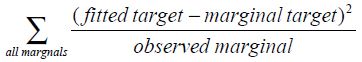
The Deming and Stephan (1940) and Deming (1943) works also included a goodness-of-fit metric, along with a procedure for optimizing it. Their measure was a chi-square-like metric:

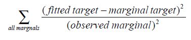
In the 1960s J. Stephens Stock, a colleague of Deming, developed a computer program for producing weights that optimize their modified measure of goodness of fit:
Unfortunately, Stock and his Market-Math Inc. partner Jerry Green never published their program but made it available to the market research community1. And it is this algorithm which is the default weighting algorithm in The Analytical Group’s WinCross.
This algorithm, and the linear and GREG weighting procedures (see Deville and Särndal (1992) and Deville, Särndal, and Sautory, (1993)) that seek to find weights which will optimize their associated criteria, may arrive at negative weights for some of the observations. This is because the data may be so inconsistent with the target marginals that the only way to reconcile the two is to create some negative weights. Dorofeev and Grant (2006, page 57) have presented an example of a weighting situation where the only possible set of weights which work include some negative weights. Their example is the following:
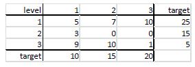
For the second row sum to be 15, the weight on cell (2, 1) must be 5. But 5 times 3 exceeds 10, so that either cells (1, 1) and (3, 1) must have negative weights in order for the first column sum to be 10.
Of course this is an unnatural example, in that there are 0s in columns 2 and 3 of row 2. But it illustrates the problem, which can occur even in perturbations of this example where the 0s are replaced by small nonzero frequencies. Mathematically, for this example we must solve six linear equations – corresponding to the six targets – for nine unknowns – the nine cell weights, with the constraint that the nine unknowns must all be positive. There are lots of solutions to this mathematical problem, of which iterative proportional fitting may converge on one, but the moment a goodness-of-fit criterion is superimposed on this problem, the imbalance of the data with the targets can show up in the form of negative weights.
The negative weights may be eliminated by the use of quadratic programming (see Schrage (2016)), an optimization algorithm invented in 1955 but not considered by either Deming or Stock as a means of optimizing their respective measures of goodness of fit. As can be seen from the above goodness of fit formulas, the marginal targets and observed marginals are constants, so that the goodness of fits are quadratic functions of the fitted target. Unfortunately, as will be seen in the example below, there may be multiple sets of weights which minimize the goodness of fit measure.
Kish (1965, Section 8.2, p. 258) coined the name “design effect (Deff)” as the ratio of the variance of a statistic under simple random sampling without replacement with a sample size of n to the variance of the statistic under the complex design with the same sample size. If the statistic is the sample mean, then the variance of the statistic is s2/n, where s2 is the variance of the population. In the case of weighted simple random samples in which the sum of the weights is n, the variance of the weighted mean is s2/ƒ, where ƒ is given by
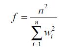
and wi is the weight of the i-th sample member. We call ƒ the effective sample size for the weighted sample. In statistical testing for equality of weighted means and/or weighted proportions, it is the effective sample size that is used in determining the standard error of the weighted mean.
We posit as a new criterion for selection of weights that of maximizing effective sample size. This criterion maximizes ƒ given above, or equivalently minimizes its denominator. Since the denominator is a quadratic function of the weights and the marginal constraints are linear constraints of the weights, the selection of optimum weights can be performed using quadratic programming (see Schrage (2016)). Using this criterion for sample balancing will both guarantee nonnegative weights and guarantee the highest possible effective sample size for the weighted sample.
An example
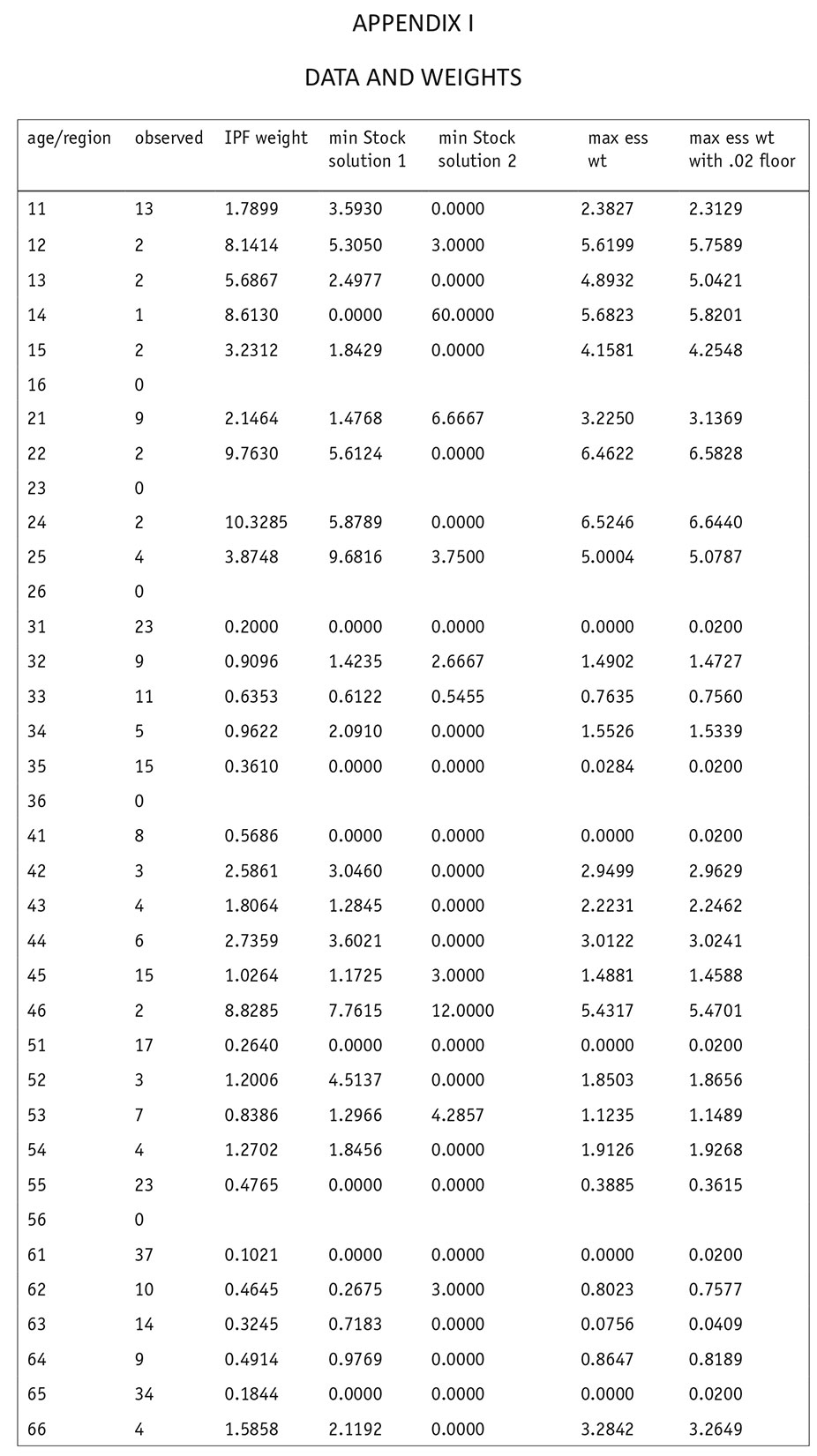
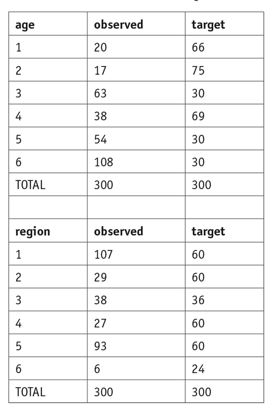
Consider for example the data in Appendix I, in which there are 300 respondents classified by age and region, and in which the observed and target marginals are shown in the following chart.
The weights produced by iterative proportional fitting (IPF), by two different quadratic programming minimizations of the Stock goodness of fit, and by maximizing the effective sample size (ess) subject to these marginal targets are given alongside the observations in Appendix I. As one can see, there are multiple sets of weights which minimize the Stock goodness of fit criterion. The effective sample size
based on IPF is 78.22 and that of maximizing ess is 95.89, a 22.6 percent gain. (The effective sample sizes of the two sets of weights exhibited that minimize the Stock goodness of fit are 75.71 and 18.82, respectively. And incidentally, quadratic programming can also find the set of sample balancing weights which produce the worst possible effective sample size, which in this case is 14.36.)
One should note that some of the cells get 0 as weights when the effective sample size is maximized. (In our example, cells 31, 41, 51, and 61 got 0 weights.) One nice feature of quadratic programming is that, instead of setting the constraints on the weights as being ≥ 0, one can set the constraints on the weights as being at least some positive number. With this modification one can still insure that the marginal constraints are met, that each cell will have a positive weight greater than some lower bound and in addition find the weights that produce the largest effective sample size. We illustrate this in Appendix I by exhibiting weights which achieve sample balancing and in which we require the weights to be at least 0.02. The effective sample size using this set of weights is 95.11, less than a 1 percent reduction from the optimal ess.
LINDO Systems Inc. has implemented a module which uses quadratic programming as described above to produce weights which satisfy the marginal constraints and produce the largest possible effective sample size. Optionally, it will find such weights all of which will be larger than a fixed minimum. This module also will find a set of weights which minimize the Stock goodness of fit.
References
Deming, W. Edwards. 1943. Statistical Adjustment of Data. New York: John Wiley & Sons.
Deming, W. Edwards and Stephan, Frederick F. 1940. “On a least squares adjustment of sampled frequency table when the expected marginal totals are known.” Annals of Mathematical Statistics, 11 (4), 427-44.
Deville, Jean-Claude and Särndal, Carl-Eric. 1992. “Calibration estimators in survey sampling.” Journal of the American Statistical Association 87 (June) 376-82.
Deville, Jean-Claude, Särndal, Carl-Eric, and Sautory, Olivier. 1993. “Generalized raking procedures in survey sampling.” Journal of the American Statistical Association 88 (September): 1013-20.
Dorofeev, Sergey and Grant, Peter. 2006. Statistics for Real-Life Sample Surveys: Non-Simple-Random Samples and Weighted Data. Cambridge: Cambridge University Press.
Fienberg, Stephen E. 1970. “An iterative procedure for estimation in contingency tables.” Annals of Mathematical Statistics, 41 (3), 907-17.
Kish, Leslie 1965. Survey Sampling. New York: John Wiley & Sons.
Schrage, Linus. 2016. Optimization Modeling with LINGO. Chicago: Lindo Systems Inc.
Footnote
1 In Public Opinion of Criminal Justice in California, a 1974 report for the Institute of Environmental Studies at University of California Berkeley by the Field Research Corp., we find a use of this algorithm, with the note (p. 118) “…the weighting correction is based on a design concept originated by the late J. Stephens Stock and Market-Math Inc. It is currently used by Field Research Organization and several other leading research organizations.”