Artificial intelligence and machine learning in market research: Part 2: Decision tree analysis

Editor’s note: David A. Bryant vice president at Ironwood Insights Group. 

In Part 1 of this article, I explored the area of cluster analysis, focusing on the k-means clustering algorithm. In this second part, I will explore the area of decision tree analysis using the CHAID algorithm.

Decision tree learning creates a visual decision tree graph as a predictive model which maps observations, or individual respondents, that help to predict an individual’s likely outcome. In medicine, decision trees can be used to predict who is likely to have a stroke or a heart attack. In finance, decision trees can be used to predict who is most likely to default on their mortgage. In customer experience, decision trees can be used to predict which customers are most likely to be unhappy and go to a competitor (churn). For this decision tree example, I am going to look at the customer churn issue and will focus on decision tree analysis using the CHAID algorithm. CHAID stands for chi-square automatic interaction detector. CHAID:

• Is commonly used in the market research industry.
• Can easily handle a large number of independent variables. 
• Is easy to understand.
• Handles missing values well. 

Decision tree analysis using the CHAID algorithm

For this example, I am going to look at 1,000 telecommunications customers¹ to see if we can find patterns within the data that will help predict which customers will churn (switch to a competitor) in the next month. The data file has 41 unique data fields that help to understand each customer. These variables include both continuous data such as months they have had service, their age and years at their current address, as well as categorical data such as marital status, level of education and whether they rent equipment or not. 

The data file has a single target variable called churn. This variable identifies whether or not the customer switched to a competitor in the past month (yes or no). When attempting to understand customer preferences and develop a customer service model, researchers usually begin by trying to identify which customers are most likely to churn. 

One of the easiest things about CHAID decision tree analysis is that to start the analysis we can simply select all 41 unique data fields as independent variables and specify the churn variable as the dependent variable. 

Because chi-square can’t be run on continuous variables, such as months of service or age, the CHAID algorithm starts the process by converting any continuous variables into deciles. CHAID will then evaluate the data and determine whether to combine some of the deciles together to better fit the data. This process is driven entirely by the data without analyst intervention.

For ease of visualizing the decision tree diagrams, I have oriented the decision tree in a left-to-right chart rather than top-to-bottom. 

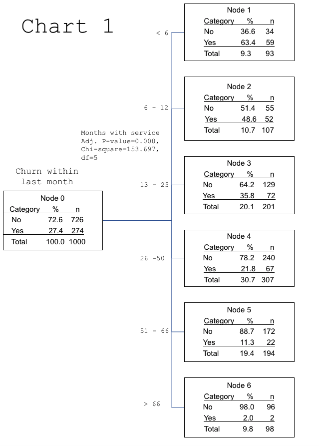
The first level of the CHAID analysis graphic is shown in Chart 1. At the left of the tree, in Node 0, you can see that overall, 27.4% of customers churned in the past month. Each node has a simple table which quickly shows the percentage of customers who did not churn in the past month and the percentage of customers who did churn in the past month. This makes it easy to identify a node that has higher than normal churn just by looking at the percentage of “Yes” in each node. 

The chi-square algorithm found that the most important variable that predicted churn was the number of months of service. In Node 1, which contains 93 customers, you can see that 63.4% of customers who have been with the telecommunications firm less than six months churned last month, compared to only 27.4% overall. Node 2 includes 107 customers who have been with the firm six-to-12 months and that 48.6% of these customers churned last month. Moving from top to bottom, the longer a customer remains with the firm, the lower the churn rate. Node 6 represents 98 customers who have been with the firm longer than 66 months and their churn rate is only 2%. 

Based on this first column in the CHAID chart, it is apparent that not all the nodes are of the same size because the CHAID algorithm has combined deciles together to form groups of customers who behave similarly. 

The CHAID algorithm will continue to go through all the independent variables to see if other variables help to explain fluctuations in the churn rate. 

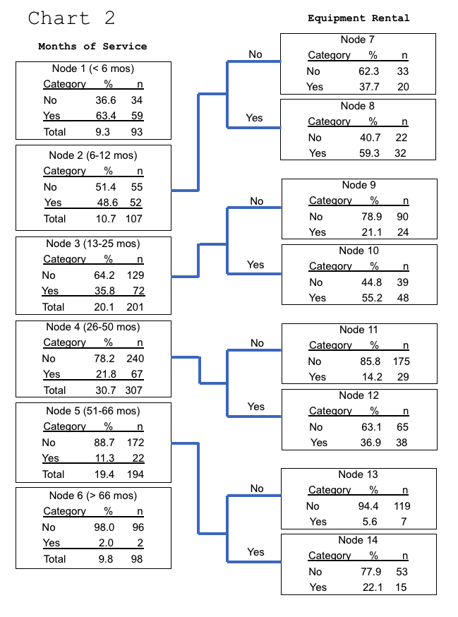
In Chart 2, the next variable that the CHAID decision tree algorithm found helpful was whether or not a customer rented equipment. 

In Node 2 the churn rate is 48.6%. But if the customers in this group rented equipment from the telecommunications firm, then the churn rate goes up to 59.3% (Node 8). 

In Node 3 the churn rate is 35.8%, but if customers in this group rented equipment, then the churn rate goes up to 55.2% (Node 10).

In Node 4 the churn rate is 21.8%, but if customers in this group rented equipment, then the churn rate goes up to 36.9% (Node 12).

In Node 5 the churn rate is only 11.3%, but if customers in this group rented equipment, then the churn rate goes up to 22.1% (Node 14).

The decision tree chart quickly shows us that newer customers are the most likely to switch telecommunications providers. It also shows us that even customers who have been with the firm six months or longer are more likely to churn if they are renting equipment.

A telecommunications firm with this type of information can easily develop client retention programs targeting their newest customers as well as customers who rent their equipment. 

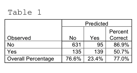
An additional result from the CHAID analysis can be seen below in Table 1. This is the classification table which looks at the data model and evaluates the accuracy of the new model. In this scenario, the results as displayed in Chart 2 will accurately predict which customers will churn 77% of the time. 

CHAID has some simple stopping rules. The first stopping rule is that a tree branch will not split unless it has at least 100 records in it. As in Chart 2, Nodes 1 and 6 were not split further because they had fewer than 100 records. 

The second stopping rule is tree depth. This is the number of levels the tree is allowed to continue until it simply halts at that maximum. The default in most software programs is five. CHAID typically wants to grow wide trees. But for most medical, financial or marketing scenarios, going beyond five levels will rarely reveal additional meaningful insights. 

The third stopping rule is confidence level, or alpha. This is the level of statistical significance that researchers desire for the purpose of the research. If the confidence level is set at .05, then the tree should grow larger. If the confidence level is set at .01, then the tree will grow less. 

Deciding how the data needs to be analyzed 

Machine learning consists of building models based on mathematical algorithms in order to better understand the data. One of the most important steps in understanding the data problem is to decide how the data needs to be analyzed in order to yield the desired results. In the grocery store example, I used cluster analysis to group the shoppers into clusters that would help us to understand the buying preferences of these shoppers. In the telecommunications company example, I used decision tree analysis to develop a prediction model to determine which customer characteristics will help predict the customers that are most likely to defect (or churn) and go to a competitor. 

While today’s machine learning algorithms make it easier to analyze large arrays of data without much programming from the analyst, it still requires that the analyst knows which type of algorithm to use for the problem and how to interpret the results. 

1. Telco.sav is an SPSS file that is supplied with the latest versions of the SPSS software.