Marketing research, AI and machine learning: Cluster analysis
Editor’s note: David A. Bryant is vice president at Ironwood Insights Group.
There continues to be a great deal of hype surrounding the use of artificial intelligence and machine learning in market research. The use of machine learning (unsupervised learning) continues to expand rapidly in today’s work environment. Some of the machine learning algorithms available to market researchers include:
- Cluster analysis – k-means, hierarchical and two-step clustering.
- Decision tree analysis – including CHAID, CRT and QUEST decision trees.
- Artificial neural networks – including multilayer perceptron and radial basis function.
In this two-part article, we will explore two of the most commonly used machine learning techniques used by market researchers: cluster analysis and decision tree analysis. In this first part, we explore the area of cluster analysis and will briefly look at the k-means clustering algorithm. In the second part, we explore the area of decision tree analysis. Specifically, we will explore decision trees using the CHAID algorithm.
Cluster analysis
Clustering involves creating groups of observations or individuals (clusters) and complying with the condition that individuals in one group differ visibly from individuals in other groups. The output from any clustering algorithm is a label, which assigns each individual to the cluster of that label.
Clustering uses an unsupervised machine-learning algorithm to identify patterns found within unlabeled input data. For example, when creating a new marketing campaign, it would be useful to segregate potential customers into subgroups based on information associated with each person to create a specific number of clusters so that the people in each cluster have similar features and demographics to each other and differ from the people in other clusters.
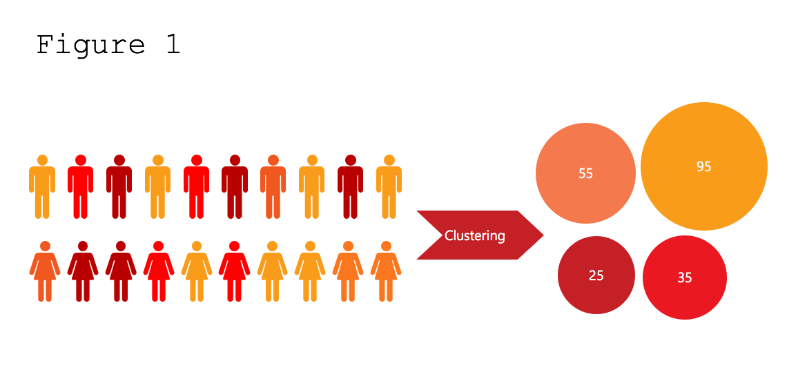
In Figure 1 we see that people are segregated into four different clusters of different sizes. One cluster has 95 people, a second cluster has 55 people, a third cluster has 35 people and the final cluster has 25 people. Individuals in each cluster may share demographic, socioeconomic or consumption patterns. The machine learning clustering algorithms will find these patterns from the data and group people together in the best way possible.

Cluster analysis and purchasing habits
In our evaluation of data using cluster analysis, we are going to look at the purchasing habits of 440 individuals over 12 months in their local grocery store. We have data collected on how much each individual spent during a 12-month period in six areas of the store:
- Fresh produce.
- Milk and dairy.
- General groceries.
- Frozen foods.
- Soap and paper products.
- Delicatessen.
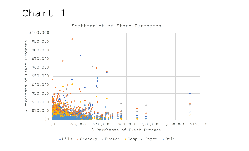
Let’s look at a scatter plot that shows the amount these 440 individuals spent in each of the six areas.
In Chart 1, we have created a scatter plot where the 12-month amount spent on fresh produce is shown along the horizontal (or X) axis in the chart. This is then matched along the vertical (or Y) axis with the 12-month amount spent on each of the five remaining types of products: milk and dairy, general groceries, frozen foods, soap and paper products and delicatessen.
By just looking at the data as displayed in Chart 1 it is difficult to identify any pattern in purchasing habits among the 440 individuals. That is where cluster analysis becomes useful.
One of the most popular clustering algorithms is k-means. K-means clustering focuses on separating the instances into clusters of equal variance by minimizing the sum of the squared distances between two points.
The k-means algorithm is used when we have data that has not previously been classified into different categories. The classification of data points into each cluster is done based on similarity, which for this algorithm is measured by the distance from the center (centroid) of each cluster. When the algorithm has completed running, we are presented with two major results:
- Every observation will have been assigned to a specific cluster.
- The centroid of each cluster will be identified.
The k-means algorithm works through an iterative process that begins with the analyst specifying a specific number of clusters to evaluate. An initial cluster centroid is randomly assigned and then all data points are assigned to the nearest cluster in the data space by measuring their distance from the centroid. The objective is to minimize the distance to each centroid. Centroids are calculated again by computing the mean of all data points belonging to the cluster. This process continues through an iterative process until the clusters stop moving. This is known as convergence of the clusters.
In our grocery market purchasing data, we initially tried two, three, four and five clusters before settling on three clusters.
In Table 1 we can see the results of the iterations of cluster centering after specifying three clusters.
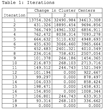
Here we see that on iteration 19 the centroids of the three clusters stopped moving and the k-means clustering algorithm reached convergence.
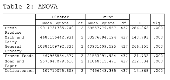
One of the statistics that we always want to look at when conducting k-means clustering is the analysis of variance (ANOVA) shown in Table 2. From this table we can see that all six measures of purchasing habits significantly contributed to the assignment of the shoppers to one of the three clusters. This can be seen by the significant F statistic for each variable, as displayed in the far-right column of the table.
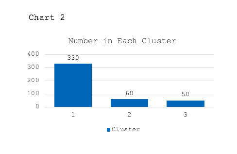
As mentioned above, one of the results of the clustering process is that each shopper is assigned to one of the final clusters, in our case, one of three clusters.
As we can see in Chart 2, most shoppers fell into cluster one, which represents 75% of all shoppers.
So how do these clusters differ and what does it tell us about the shopping habits of these 440 individuals? To help us with that, we now look at the final cluster centers for the six product types. This can be seen in Chart 3.
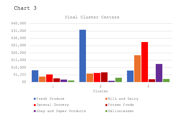
From Chart 3 we see the different purchasing habits of the three cluster groups.
Cluster one, which makes up 75% of all shoppers, spends about the same amount of money across the six product types. They purchase slightly more fresh produce and general grocery during a typical 12-month period.
Cluster two, which makes up 14% of all shoppers, spends significantly more in the fresh produce section of the grocery store. As we can see in the chart above, the average shopper in cluster two spends more in the produce section of the store than in the entire rest of the store combined.
Cluster three, which makes up 11% of all shoppers, spends more in the general grocery section of the store as well as the milk and dairy section of the store.
From the chart above we might come to the following conclusions:
Cluster one is made up of shoppers that are looking to get the best deal on all of their shopping needs. These types of shoppers are likely to frequent “big box” discount warehouse stores (such as Costco or Sam’s Club) for the bulk of their shopping needs.
Cluster two is made up of shoppers who want to prepare mostly fresh produce for their family. These shoppers are going to frequent stores with the best selection of fresh produce.
Cluster three is made up of shoppers who spend most of their money purchasing general groceries along with milk and dairy products. These shoppers are going to frequent grocery stores where they can purchase a large selection of different products in a single location, such as Walmart.
Finding patterns in data
As we have demonstrated, clustering algorithms allow the computer to sort through scores of attributes and thousands of observations to find the best way to organize the data into homogeneous groups or clusters. The algorithms can do this without much input from the analyst. Machine learning algorithms are a robust way to find patterns in data which the analyst would never discover.