Editor's note: Jeff Monroe is a Memphis, Tenn., market research manager.
Much has been written about price elasticity, revenue optimization and the impact on profitability. There is little doubt that pricing has the greatest impact on company profits. An often-cited study by McKinsey (“Average economics of 2,500 companies”) demonstrated the impact that various decisions would have on the bottom line: a 1 percent reduction in fixed costs improves profitability by 2.3 percent; a 1 percent increase in volume will result in a 3.3 percent increase in profit; a 1 percent reduction in variable costs will prompt a 7.8 percent rise in profit; but a 1 percent hike in pricing can boost profitability by 11 percent.
The objectives here are to review how revenue optimization is traditionally applied, for single and multiple products and/or services, and describe an improved multivariate approach to revenue optimization.
The multivariate model allows for identification of volatile causative forces of demand in addition to price. This not only improves modeling of short-term volatility but, more importantly, provides an inflection point indicator for short- and longer-term analysis.
To begin, an example of optimal price calculation for a single product is provided. Next, a two-product optimum with constrained supply is reviewed. Finally, a description of multivariate modeling applied to price elasticity is provided; and an approach not too distant from market-mix modeling, albeit more direct for the resource restricted analyst, is proposed.
In an effort to make this method as translatable as possible, assumptions are made to avoid a partial differential equation solution. The benefit of a streamlined process in this technical subject more than offsets the small inaccuracies experienced when applying calculus and linear algebra as opposed to differential equations. A straightforward process lets the analyst apply the model with minimal effort and provides for efficient critique by management. The solutions presented here will move the decision maker in the right direction and will be basic enough for an analyst with basic math skills to apply.
Assumptions are:
(1) the demand curve is downward-sloping; that is, the higher the price relative to other products or services, the less customers purchase;
(2) the demand curve is continuous;
(3) the result is non-negative, p ≥ 0, simply meaning you can’t have a negative price; and
(4) the demand curve is differentiable and smooth with a well-defined slope, allowing use of calculus and linear algebra instead of differential equations.
Basic price optimization - unconstrained, single product
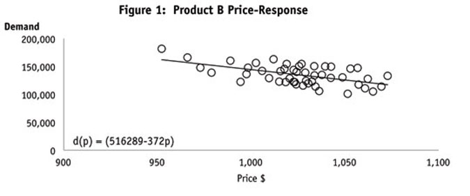
Example 1: Suppose a hypothetical company, Acme, a manufacturer of products used in housing construction, is looking to set the price of its commodity product for the current period. The company’s unit production cost c is a constant $700 per unit and the demand for the current period is governed by the linear price-response function (Figure 1):
d(p)=(516,289-372p)
This means that the demand for the product will be 516,289-372p for prices between $0 and $1,388 and that the demand will be 0 for prices over $1,388. Solving for the optimal price p*:
516,289-372p*=372(p*-700)
p*=$1,044
At the optimal price of $1,044, total commodity product sales will be 128,000 units, total revenue will be $133,662,540 and total contribution will be $44,062,237.

A question that often arises is how to best determine the price-response function. Ideally, market research will provide direction, testing for volume indicators from customers at different price points. Unfortunately, this is not always possible and research is expensive and may take months to complete. In the absence of research, a price-response function may be derived using historical data, plotting historical price against volume. An in-depth discussion of the statistics involved is beyond the scope here. In economic terms, the price-response function is referred to as the demand curve. Some economic literature applies an inverted demand curve, which is simply a linear equation with volume on the y-axis and price on the x-axis. An obvious problem with the model above is that it fails to consider other products in the market and the reality that supply is limited. The following example tackles both issues.
Revenue optimization for two products under constrained supply
Example 2: Suppose Acme Company is now looking to optimize prices for two of its products simultaneously and is supply-constrained to 128,000 units per period. The first item will be referenced as Product B and the second item Product C. Product B is of better quality than Product C and customers appear willing to pay more for it. Acme wants to find just how much more customers are willing to pay. Cost, c, for Product C is $650/unit, and the cost of Product B is $700/unit. Acme needs to find the optimal price for both products under constrained supply.
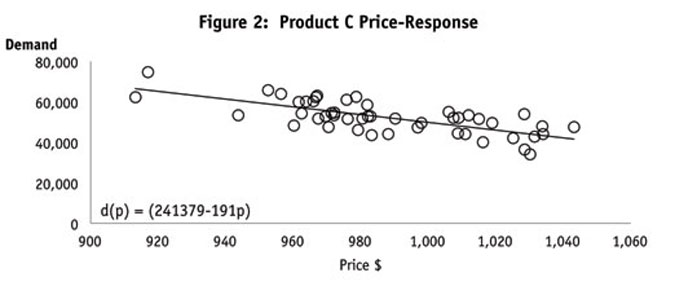
It is determined the price-response curves are (Figure 2):
Product C: dc(pc)=(241,379-191pc)
Product B: db(pb)=(516,289-372pb)
The aggregate demand curve is therefore:
d(p)=(241,379-191p)+(516,289-372p)=757,668-563p
This means that the demand for Products B and C will be 757,668 - 563p for prices between $0 and $1,345 and that demand will be 0 for prices over $1,345. The optimal price (p*) is $1,122.
Thus, the optimal price for both products is $1,122. At this price, the company will sell exactly its capacity of 128,000 units, grossing $143,593,709.
Now, comparing differential pricing based on the assumption that the company can charge more for Product B than for Product C, Acme needs to find the optimal price for each product, which requires solving the constrained optimization problem:
maximize pc(241,379-191pc)+pb(516,289-372pb)
subject to pc(241,379-191pc)+pb(516,289-372pb)≤128,000
The marginal revenue for Product C is 2pc - 1,260 and for Product B the marginal revenue is 2pb - 1,388. Equating the two marginal revenues, 2pc - 1,260 = 2pb - 1,388, gives pb = pc + 64. In other words, the price for Product B will be $64/unit higher than the price for Product C.
The other condition that must be satisfied is that the total demand for both products must be equal to capacity; that is (241,379 - 191pc) + (516,289 - 372pb) = 128,000. Solving both conditions simultaneously gives pc = $1,076 and pb = $1,140. At these prices, Acme will sell 35,429 units of Product C and 92,571 units of Product B, thus selling at full capacity of 128,000 units. Revenue generated will be $143,593,709, and total contribution will be $55,764,858.
It is important to note, and it is often the case, that optimizing multiple products, rather than each product singularly, results in higher revenue and contribution. In this example, Acme receives $9,931,169 additional revenue compared to the first example and $11,702,620 additional contribution. The economics behind this is sound. Because Acme is optimizing two products simultaneously, it is better able to price its products along the entire aggregate demand curve, rather than just a portion of it.
Multivariate revenue optimization
In the previous examples, the assumption was that volume was entirely price-related. That is to say, that volume was due solely to price and nothing more than price. While this may be accurate in the long run, pricing decisions are rarely made over the long run. Instead, price decisions are usually made monthly, weekly or even daily, depending on the industry and market. While there is little doubt that price is, for most products, the most important factor driving a consumer to a decision, it is rarely the only factor. Thus, to accurately form a price-response function, the traditional price elasticity model is inadequate.
A second argument against expanding the price-response function to a multivariate model is that over time, all other variables are ultimately reflected in either price or demand. The issue arises however, when a market is at an inflection point in the historical price-demand relationship or short-term volatility goes unaccounted for in the long-term price-demand approach; a situation made all too familiar by the recent recession.
Example 3: Acme Company has determined that housing starts is a very good indicator of the demand for its products. So Acme adds housing start variables to the price response functions:
Product C: dc(pc)=(180,785-151pc+31hc)
Product B: db(pb)=(559,989-401pb+20hb)
Note that the above shows, as expected, an inverse relationship between price and demand and a positive relationship between housing starts and demand. This is expected. If this were not the case, caution should be made in using the additional variable applied. It should go without saying that the normal statistical procedures should be conducted to ensure the variable being added is truly a good measure of demand.
Equating the above and constraining to 128,000 units of capacity results in an optimal price for Product C of $1,037 and for Product B of $1,136. As shown in Figure 3, 24,110 units would be sold of Product C and 103,891 units of Product B. Revenue is $143,056,695 and contribution is $54,661,887.
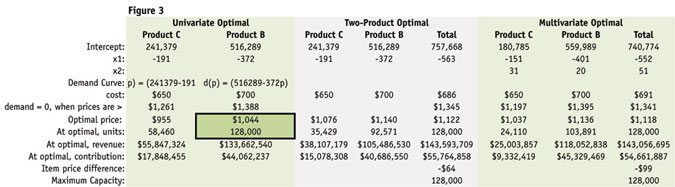
When comparing the previous example with the multivariate approach, it is interesting to note that while revenue and contribution remained mostly the same, the product mix shifted much more toward Product B. In fact, the pricing for Product B held more its price, only declining $4/unit compared to the previous example. The Product C declined $39/unit. The suggestion here is that without a model that more completely describes the market, Acme may be overpricing its Product C, in addition to expecting much greater volume than reality may dictate. Ultimately, an improved model will lead the analyst to advise the business in a more knowledgeable way, resulting in improved demand and financial forecasts, as well as better use of company resources.
References
Phillips, Robert., L. Pricing and Revenue Optimization. Palo Alto, Calif.: Stanford Business Books 2005: 104-105.
U.S. Department of Commerce: Census Bureau/FRED. http://research.stlouisfed.org/fred2/
McKinsey and Company. “Average Economics of 2,500 Companies.”