Editor's note: Tim Bock is CEO and founder of Sydney-based software firm Displayr.
If you’ve studied a bit of statistics or machine learning, you’ve probably come across logistic regression. Logistic regression is an approach to building a predictive model for an outcome with two categories. For this reason, it is also called binary logit. For many years, logistic regression has been the standard approach to building these types of models – and if you are a trained statistician with a lot of extra time, it’s a great technique. However, if you are anyone else, it is confusing and hard to interpret. Logistic regression has been superseded by various machine learning techniques, including random forests, gradient boosting and deep learning – and even the humble decision tree. Although logistic regression has long been considered a gold standard, even the simplest of decision tree algorithms – CART – is generally superior to logistic regression.
The main drawback of logistic regression is that it is difficult to correctly interpret the results. It is important to note that decision trees are not necessarily statistically superior to logistic regression. It is not their technical precision which makes them better than logistic regression but rather their clarity and ease of use. The most statistically precise model in the world is useless if the people who need to interpret it are unable to do so.
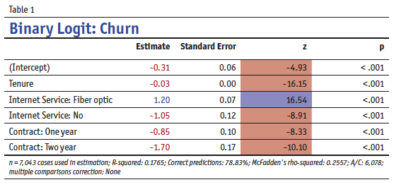
To illustrate this point, consider the logistic regression output shown in Table 1. This model uses an IBM data set (https://bit.ly/2rp5vwj) and aims to predict whether or not customers churned. Even the most experienced statistician cannot glance at Table 1 and quickly make precise predictions about what causes churn.

By contrast, a decision tree based on the same data makes interpretation far easier (Figure 1). It shows how the other data in the dataset predicts whether customers churned.
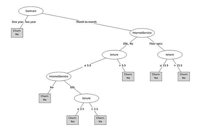
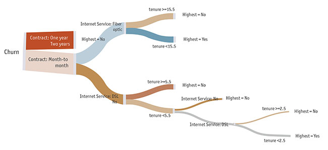
This is a typical visualization of a decision tree. It is already far easier to read than the logistic regression. However, we can improve it even more by visualizing the tree using a Sankey diagram. While this is not the most common way of visualizing decision trees, I would argue that it is the best way, due to its clarity of interpretation (Figure 2).
You can view an interactive version of this tree, and the underlying code, at https://bit.ly/2BWWzob (registration required).
From this decision tree visualization, we can easily draw several conclusions:
- The single best predictor of churn is contract length. We know this because it is the first split in the tree.
- People with a month-to-month contract are different from those with a one- or two-year contract. CART trees always split into two categories. The fact that one- and two-year contracts have been combined means that the difference between these two groups is less than their difference to month-to-month. It does not necessarily mean that there is no difference between one- and two-year contract people in terms of their propensity to churn – it just means that this difference is smaller than that between annual and monthly contracts. The decision tree could, if the data warranted, split people further on in terms of one- and two-year contracts.
- People with a one- or two-year contract are less likely to churn than those with a month-to-month contract. This is indicated by the text on the tree, as well as the color shading – more blue means more likely to churn and more orange means less likely to churn. In the interactive version of this visualization, you can hover to see the underlying data, which indicates people on a one- or two-year contract have only a 7 percent chance of churning.
- More people are on a month-to-month contract than are on an annual contract. We know this because the corresponding “branch” of the tree is thicker. We can also see the number of people by hovering over the node.
- If we know somebody is on a one- or two-year contract, we can already conclude that they are unlikely to churn. The predictions of the model do not require splitting this branch further.
- Among the people on a one-month contract, the best predictor is their Internet service, with people on a fiber optic service being much more likely to churn.
- Among people with a month-to-month contract who have a fiber optic connection, they are likely to churn if their tenure is 15 months or less (69 percent), whereas those on the fiber optic plan with a longer tenure are less likely to churn.
In this manner we can continue explaining each branch of the tree.
Make mistakes
The problem of logistic regression being difficult to interpret should not be taken lightly, as it is actually more serious than it may initially appear. People trying to build a model which they are unable to correctly interpret are likely to make mistakes. Furthermore, they are unlikely to notice when something is amiss with their model. This leads to a snowball effect, whereby they inadvertently create a faulty model which they then go on to misinterpret.
The complexity of logistic regression makes this a real possibility. To use them correctly, you need to constantly ask yourself a lot of questions: Are you using feature engineering to ensure that the linear model isn’t a problem? Did you use an appropriate form of imputation to address missing data? Are you controlling your family-wise error rate or using regularization to address forking paths? How are you detecting outliers? Are you looking at your G-VIFs to investigate multicollinearity?
With so much to juggle, it’s unlikely that anyone other than a trained statistician will be able to correctly use logistic regression with the precision required to draw solid conclusions.
The wonderful thing about decision trees is that they really are as simple as they appear. You can use them and interpret them correctly without any advanced statistical knowledge. All that is really required to be successful is common sense.
More accurate predictions
You may be thinking that the reason logistic regression is better known than the decision tree is because it makes more accurate predictions. Perhaps surprisingly, this turns out not to be the case! With the data set used in this example I performed a test of predictive accuracy of a standard logistic regression (without taking the time to optimize it by feature engineering) versus the decision tree. When I performed the test I used a sample of 4,930 observations to create the two models, saving a further 2,113 observations to check the accuracy of the models. The models predicted essentially identically (the logistic regression had 80.65 percent accuracy and the decision tree had 80.63 percent).
My experience is that this is the norm. This is of course not always the case – some datasets do better with certain models, so it is always wise to compare multiple options. If your focus is solely on predictive accuracy, you would generally be better off using a more sophisticated machine learning technique (such as random forests or deep learning). However, given the superiority of the decision tree in terms of ease of use, I would argue that it is usually the safest option.
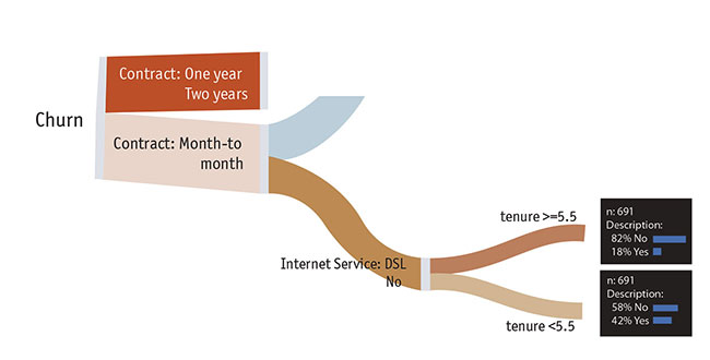
So why, then, are logistic regressions better known than decision trees? Unfortunately for decision tree enthusiasts like myself, logistic regression does certain things a lot better than a decision tree can, if you have enough time and expertise. As an example, consider the role of tenure (Figure 3). The decision tree tells us that if somebody is on a month-to-month contract, with DSL or no Internet service, the next best predictor is tenure. People with a tenure of less than six months have a 42 percent chance of churning, while people with a tenure of six months or more only have an 18 percent chance of churning. As far as predictions go, this is a bit blunt. It is unlikely that six months is the magical cutoff when people suddenly become far less likely to churn. It is more likely that the chance of a customer churning drops slightly with each additional month. A drawback of the decision tree is that it simplifies these relationships. Logistic regression can, with appropriate feature engineering, better account for such a relationship.
Decision trees are also very expensive in terms of sample size. Every time the tree splits the data using a predictor, the remaining sample size reduces. Eventually it gets to a stage where there is not enough data to identify further predictors – even if some of these predictors are relevant. This means that decision trees are not a good choice for small sample sizes. By contrast, logistic regression examines the simultaneous effects of all predictors.
However, the flip side is that decision trees are much better when effects are sequential, not simultaneous. This is the case with the example shown in this article. If somebody is on a contract, they are locked in and therefore other predictors of churn are likely not relevant. The decision tree correctly shows this relationship, whereas a typical logistic regression would incorrectly consider all predictors to be equally relevant. In cases like this, decision trees make substantially more sense.
A further weakness of decision trees is that they have their own potential for misinterpretation: many people assume that the order with which predictors appear in a tree is indicative of their importance. This is often not the case – the only prediction in which the order is meaningful is the first one. If there are two highly correlated predictors, only one of them may appear in the tree – and which one it is will be a bit of a fluke.
The upshot of all this is: If you’re doing an academic study and want to make conclusions about what causes what, your best bet is probably logistic regression. However, if your goal is either to make a prediction or describe the data, logistic regression is often worse than a decision tree.
Other options
There are many different algorithms for creating decision trees. In this article I have used a classification tree; however, there are countless other options that can also be used.
When creating a decision tree, a choice needs to be made about how big the tree will be. If your goal is to replace logistic regression with a decision tree, you can maximize the predictive accuracy of your tree based on cross-validation. On the other hand, if your goal is to describe the data, it can be useful to either create a smaller or larger tree.
The key point to take away from all this is that we don’t build models just for ourselves – they have to be accessible for the people who need to interpret them. If either you or your audience don’t have the technical skills to correctly interpret logistic regression, decision trees are a far safer option, one with which you have a greater chance of success.
So, next time you’re dreading trying to explain your logistic regression model, try using a decision tree instead!