Decoding the drivers of brand equity

Editor's note: Jayant Rajpurohit is lead consultant at Absolutdata Technologies Inc., Alameda, Calif. Aaroshi Asija is a consultant with Absolutdata Technologies Inc., Gurugram, Haryana, India.

Marketing professionals face many challenges when seeking to adapt their brands to shifting consumer trends and needs. With the ever-changing competitive scenario, your brand is at a constant risk of being eliminated from the customer’s mind, which puts a lot of questions in front of the brand manager/marketer:

How do we keep the brand up to date? Is the brand performing well on attributes that are currently of value to consumers/users? Are the attributes that influence brand equity changing? 

What marketing levers are available to work with? What tangible and functional attributes can the brand activate? How do we activate emotional attributes such as trust?

What’s the best mix of marketing resources? Is the brand equity driven by attributes of campaign (awareness), innovation (uniqueness and variety), messaging/copy (softer emotional and perceptual attributes), channel (point of purchase), pricing (value for money), etc.?

Is the brand winning against the competition? Is it performing well compared to competition on the attributes that matter?

All these questions have roots in a larger one: How are functional and emotive brands driving the brand equity in the market? For a traditional driver analysis, we could sift through different attributes and identify which ones need investment through campaign (awareness), innovation (evolving needs/changing drivers), packaging (usage experience attributes) or pricing (value for money). But this is easier said than done, as a traditional driver analysis does not provide all the answers for the above questions.

The aim of a traditional driver analysis is to identify the drivers of brand equity rather than how these attributes are driving brand equity. The most simplistic driver analysis gives the marketer an understanding of where his/her brand stands in the market on the most important brand attributes but it would be unable to precisely measure questions around the following areas:

Tangible versus intangible. Soft attributes like perception of the brand (such as trustworthy, youthful, a leader, calm, etc.) are difficult to act upon. If these come up as important attributes, how do you find out which tangible attributes contribute to the softer attributes? Can a soft attribute be tied quantitatively to a tangible metric, e.g., can trust in a food product be quantitatively measured through the presence of organic ingredients or the fact that it was recommended by friends and family, etc.?

Interlinkages. The real measure of an attribute is not just its relative importance calculated through beta coefficients of key driver analysis (as shown in Figure 1) but through other indirect impacts it has on other attributes as well. Hence, we need to understand how these attributes connect or impact each other.

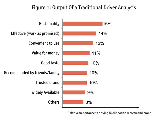
What constitutes true brand equity in the market? A traditional driver analysis uses regression as a technique to identify the key drivers of brand equity. In this process the survey responses for the brand perception attributes are input as independent variables. But there is always a necessity to define a metric (read: brand equity) as a dependent variable, against which the regression will run, thus creating a burden to use proxies for brand equity for the dependent variable, e.g., in Figure 1 it is likelihood to recommend the brand. Sometimes a combination of CSAT, likelihood to recommend and likelihood to repurchase is also used. These proxy metrics are stated responses from the survey, hence the regression is not for drivers of brand equity but for these stated variables (which are assumed to represent brand equity). Structured equation modelling doesn’t require this necessity of a dependent variable but rather produces a brand equity metric as a latent variable.

Solve for the drawback

If we could regress (or model) the attributes (both emotional and functional attributes and other metrics such as awareness, recommendation etc.) without the need for a predefined or calculated dependent variable (similar to Bayesian models, where latent variable definition suffices if we have a list of independent variables; we’ll explain latent variables later in the article), we would be able to solve for the drawback of traditional driver analysis. This can be achieved through partial least squares modelling, where brand equity is our latent variable, i.e., it doesn’t exist as a number, but all variables would interlink and model towards driving this final dependent variable. 

Brand health trackers capture customer perceptions through different salience measures across all respondents. Trackers also measure satisfaction and recommendation among users but when these metrics are used as dependent variables, they exclude non-users. Our framework was designed to best capture the essence of two customer groups – user and non-user. A user would have knowledge about the brand based on its current/past usage, whereas a non-user would have limited experience with the brand and the brand’s equity would largely be driven by perceptions. Hence when modelling we need to separate the datasets for the two populations.

We arrived at the brand equity score with the help of partial least squares (PLS) regression. PLS multivariate regression is a variance-based structured equation modeling (SEM) technique that gave us the flexibility and robustness needed to merge these two models of users and non-users. 

SEM establishes the relationship of cause and effect between different variables. One of the outputs – path diagrams – shows the variables interconnected with lines that are used to indicate causal flow (i.e., it establishes cause-and-effect relationships between variables). Structured equation modelling is an umbrella term encompassing several statistical methods to achieve the similar outcomes. Unlike other SEM techniques, PLS:

• accounts for dependent variables which may not be quantified (i.e., we do not have the final brand score available in the raw data for each respondent);
• considers the indirect effects of independent variables, i.e., not only does it establish the impact of a variable on the latent variable (for example, brand equity) but it also measures the indirect impact through interlinkages;
• constructs the model with many interrelated predictors/variables.

PLS regression calculates the value of a latent variable (brand equity score) from indicators (independent variables) after multiple iterative regressions at the back end. The model ensures that the calculation of dependent variables would also be a function of inter-collinearity between independent variables.

PLS is available as an open-source package on R (plspm library) and other platforms as well. In this article, we focus on its advantages and interpretation and offer a use case for marketing research in brand equity.

Two main outputs

There are two main outputs of a PLS model through R: path diagrams and the impact of independent variables (attributes) on brand equity (indirect and direct).

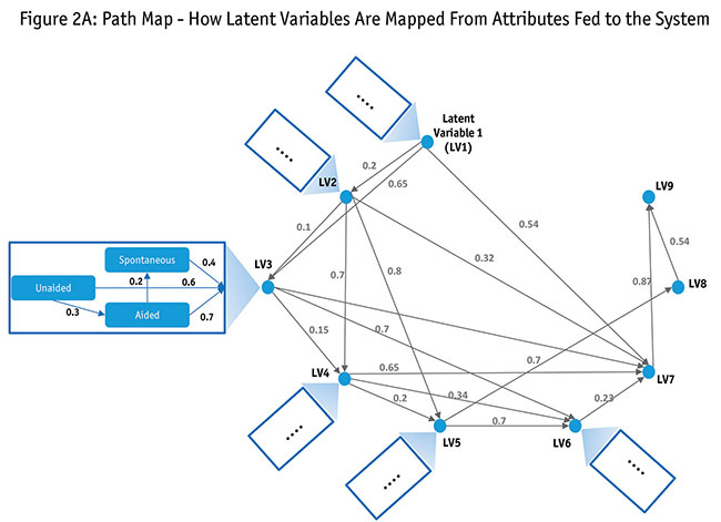
Path diagrams. The chief strength is expressed in path diagrams, allowing clients and researchers to better understand the output. The path diagram takes the individual attributes and creates several latent variables. Each latent variable is a factor of several individual attributes that were tested in the survey. The output shows us the relationship of these latent variables with the attributes and with each other but it does not help us name them for a linear understanding. This is where we need to bring in business sense and name these latent variables. In Figure 2A we show a condensed map of latent variables with the relationship to one another. To illustrate how individual attributes make these latent variables we show the impact and contribution of aided, unaided and spontaneous awareness in driving a latent variable (LV3). This latent variable, in turn, impacts several other latent variables, which in turn impacts brand equity. 

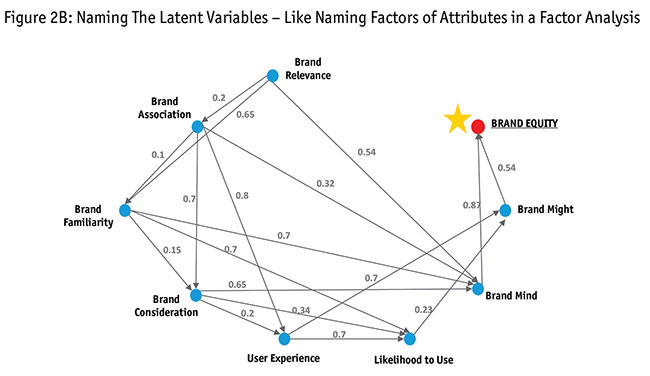
Both Figures 2A and 2B explain the journey of getting latent variables from attributes/input variables and naming them. In Figure 2B we illustrate the journey of naming these latent variables. Just like we named latent variable 3 “brand familiarity,” we name the other variables based on their input variables. Like brand perception, familiarity and word of mouth play big roles, as does user experience, in determining a brand’s position in a customer’s mind. Our framework was set to translate these softer variables into an index that could be tracked over time. You will notice that latent variables 7, 8 and 9 do not have any significant attributes contributing to them. Figure 2B refers to them as brand mind and brand might, respectively. We clarify this dilemma below.

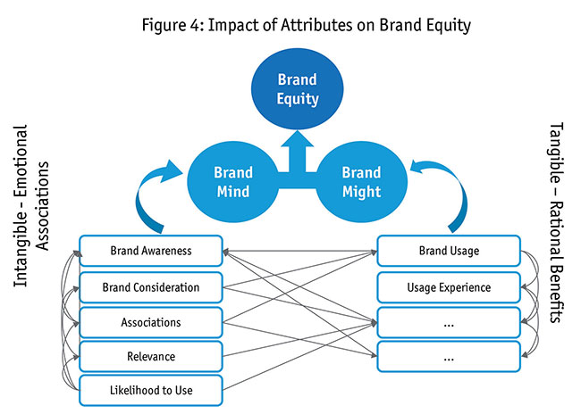
How to name latent variables driven by other latent variables. We looked at the latent variables feeding into latent variables 8 and 9. Figure 3 explains this in a flowchart. In summary, brand mind and brand might are latent variables. Looking at them, we could see emotive attributes such as perceptions of a brand as a “leader in the market,” as innovative, fun, “a brand for me” and likelihood to use, and hence decided to use the term “brand mind.” Functional attributes such as brand awareness, user experience such as CSAT, repurchase, frequency of usage, etc., would impact a latent variable, showing the might of the brand in the marketplace. We named this “brand might” (its actual power in the life of the consumer) and together with brand mind it made brand equity.

Evaluating impact. You can calculate the impact two ways. One way is a direct multiplicative model to understand the relationship between individual attributes with brand equity; the other is calculating the single brand equity number. 

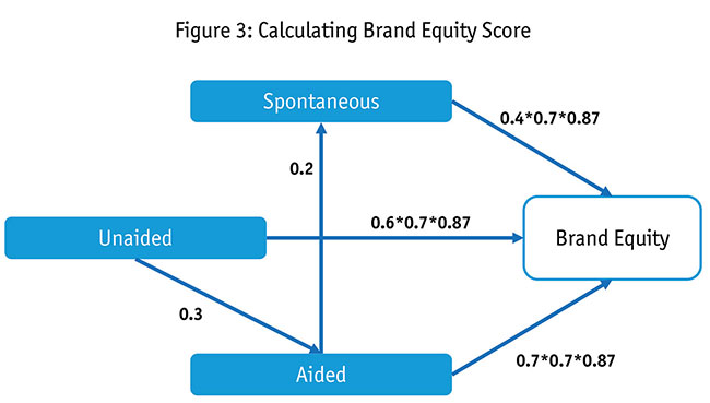
Direct multiplication. Going beyond stated awareness level, we calculate the impact of spontaneous awareness versus aided awareness in driving brand equity. You can clean the map by choosing specific attributes and calculating the impact on specific latent variables. For illustration, we chose the example of calculating the impact of awareness on brand equity. Here the impact of spontaneous awareness is multiplied by contribution of LV3 (i.e., brand familiarity) to LV7 (brand mind), further multiplied by the impact of LV7 to brand equity. This would be the next impact of spontaneous awareness (as shown in Figure 4).

Constructing one equity number. You can also bring together a host of independent variables and create a path for them to formulate one composite score, which can be tracked. Our framework calculated a brand equity score, which was defined with the help of the equation below. You would calculate the latent variables through the attribute scores which in turn would calculate the brand equity score. The equity score is indexed for tracking and ranges between 0 to 100. It can be measured for each respondent, for each brand. It is comparative, linear and relative in nature. An equity score of one brand can be compared to another like any score on a scale. Here is an illustrative equation using the path diagrams shown in Figure 2B:

Brand Equity = 0.87 x Brand Mind + 0.54 x Brand Might

Brand Mind = 0.54*Brand Relevance + 0.32*Brand Association + 0.7*Brand Familiarity + 0.65*Brand Consideration

Brand Might = 0.23*Likelihood to Use + 0.7*User Experience

Strength of an attribute

Using a path map, we know which other attributes are impacted by a certain attribute. These path diagrams can then be analyzed as shown in Figure 3. Using interlinkages, we could calculate the actual strength of an attribute versus a traditional key driver analysis (KDA). 

Traditional KDAs overestimate the importance of some attributes that emerge as key drivers through regression. And these results may change dramatically every time you run the regression on a new data set due to sampling error (e.g., latest survey data versus old survey data). Our approach solves both these problems, hence the results are more believable to the audience. The results don’t change dramatically over time (if we do the survey every year or on regular intervals) and also provide a detailed path map illustrating what other attributes are contributing and influencing a key driver. Also the results don’t change dramatically.

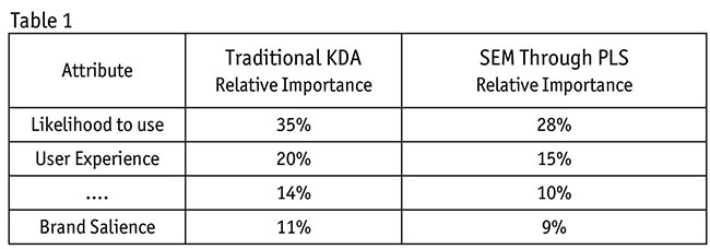
Table 1 shows how results from traditional KDA are different from SEM results. It shows the difference in the relative importance. The ones calculated by PLS are much more stable and accurate (we know this because we can trace the composition variables for each variable as described in Table 1).

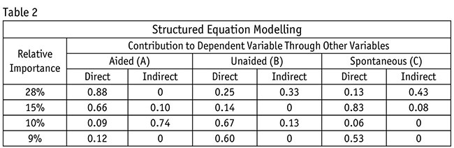
You can also do a crosstab of direct and indirect impacts. Table 2 shows how the PLS equation allows the researcher to know the impact that aided, unaided and spontaneous variables have on different attributes. The contribution table essentially states the coefficients for each variable. This can be further converted into individual equations. And this can be done for all variables in the path map (Table 2).

Traditional regression would have its beta coefficients moving drastically for every iteration with new survey data coming in. This is because it accounts for collinearity but does not lay out the map of the interlinkages. Through structured equation modelling using PLS regression we can see these interlinkages and calculate the relative importance (which doesn’t change as new data appears).

A further advantage is that this exercise can be run using the existing brand health tracker data and needs no new data collection. We can combine data of past waves of trackers to ensure a robust model with large data set.

We do not recommend executing a PLS-based structured equation model for every wave of the brand health tracker but it should be conducted at frequent intervals to ensure that the brand tracker is measuring the health of the correct metrics. Further, it strengthens the ability of marketing professionals to act on the findings.

As a rule of thumb, we recommend that the structured equation modelling for brand equity should be revised at the same frequency as segmentation. For example, if it is a highly evolving market where the segmentation is revised every two years or less, the same frequency should be applicable for the brand equity model. 

This technique has been applied with success and has confirmed acceptability in three main business-to-consumer industries:

• Subscription-based models (print and content-streaming). Brand equity is prime in ensuring subscriptions, clicks and landing on Web pages. Here the model also validated some of the missing consumer nuances that the attribution modelling using digital data was unable to provide, e.g., which messaging trait enticed consumers to click through one service over another, etc.
• Consumer packaged goods. Softer attributes such as trust, youthful, premium, exciting and friendly always come up as important in brand perception but marketing professionals struggle to associate these with packaging, user experience, value for money, availability and type of influencers.
• Hospitality (hotels and cruises). Since interlinkages of attributes are very high in this industry, things such as value for the money could be quantified through their connections with other attributes and offerings by the hotels/cruise lines.

Apart from these, the technique has also seen traction with a business-to-business case of a consulting firm trying to understand its equity versus other premium consulting firms. In each case the technique has helped the organizations realign their priority brand attributes and learn the levers of brand equity in the market.