Marketing research, AI and machine learning: Artificial neural networks

Editor’s note: David A. Bryant is vice president at Ironwood Insights Group. 

Earlier this year, I wrote a two-part article covering machine learning techniques – cluster analysis and decision tree analysis. This article will cover a third machine learning technique that is commonly used by market researchers: artificial neural networks (ANNs). 

Artificial neural networks

The two types of ANNs that are frequently used in market research include multilayer perceptron and the radial basis function. Each has their differences and advantages.

• The output of a radial basis function network is always linear, whereas the output of a multilayer perceptron network can be linear or nonlinear. You need to determine the type of problem you are trying to solve before selecting the type of ANN you want to use.
• Multilayer perceptron networks can have more than one hidden layer, whereas a radial basis function network will only have a single layer. Having more than a single hidden layer can be important when working on nonlinear problems.

In this article I am going to focus on the multilayer perceptron function because of its ability to solve linear and nonlinear problems. I will avoid going into too much detail regarding the mathematics involved in calculating the neuron weights in a multilayer perceptron (MLP) model.

Two examples of scenarios using the multilayer perceptron procedure include:

• A loan officer at a bank wants to identify characteristics that are predictors of people who are likely to default on a loan and use those predictors to identify customers who are good and bad credit risks. 
• A customer retention manager at a telephone company wants to identify characteristics that can predict which customers are most likely to switch telephone plans in the near future. This is the scenario that I discussed when exploring the decision tree algorithm in my previous article. The CHAID decision tree algorithm identified “months of service” and whether the customer “rented equipment” as the two strongest predictors of who would switch telephone companies in the near future. 

Let’s explore the multilayer perceptron algorithm using telephone customer churn data.¹ 

Understanding a multilayer perception model 

ANNs use an unsupervised machine-learning algorithm to identify patterns found within unlabeled input data. The MLP procedure produces a predictive model for one or more dependent variables based on the values of the predictor variables. The MLP procedure is robust because the dependent variables and the predictor variables can be categorical or continuous or any combination of both. 

Figure 1 shows that every multilevel perceptron consists of three types of layers – the input layer, the output layer and the hidden layer. The hidden layer can consist of one or more layers of neurons.

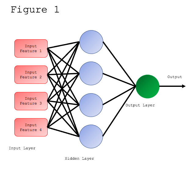
The input layer receives the initial data to be processed. The required task, such as a forecast of who will leave the telephone company in the near future, is performed by the output layer. The hidden layers of neurons are the true computational engine of the MLP. 

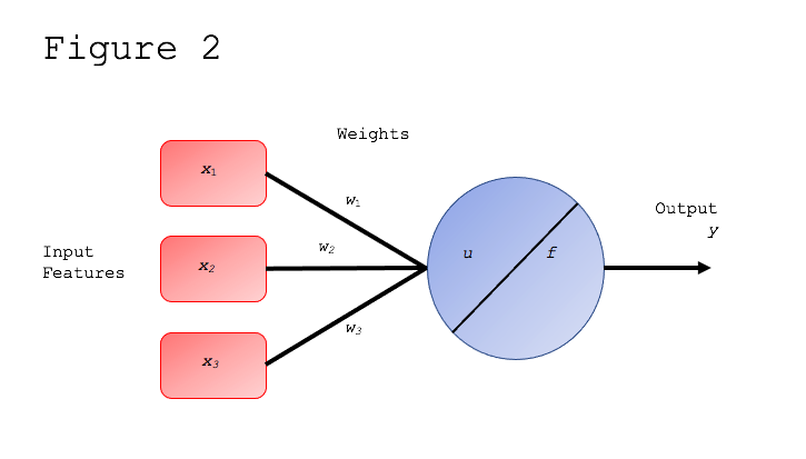
MLPs are composed of neurons called perceptrons. So, before going any further, we need to understand the general structure of a perceptron. Figure 2 shows that a perceptron receives n features as inputs (x = x₁, x₂, ..., x_n), and each of these features is associated with a weight. 

Input features must be numeric, so a categorical feature (variable) must be converted to numeric ones in order to use a perceptron. For example, a categorical feature with three possible values is converted into three input features by creating three dummy variables indicating the presence/absence of each value. 

Let’s assume that the telephone company has three levels of service – basic service, plus service and total service. So, if we want to include this categorical variable in our MLP predictor model, this input feature will need to be converted into three dummy variables. The SPSS neural network algorithm automatically makes this transformation . 

Development of a prediction model

To start the creation of our MLP predictor model we are going to begin with the two variables that came out of our CHAID decision tree model in my previous two-part series: 

• Months of service (tenure).
• Equipment rental.

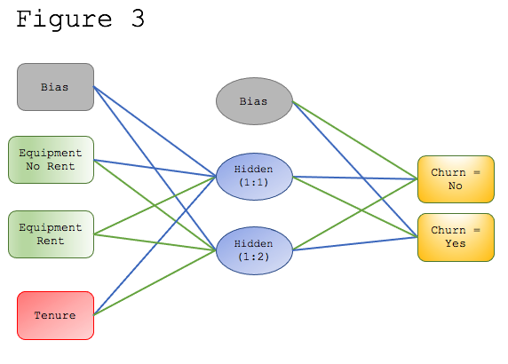
The resulting MLP appears in Figure 3.

To train and test our MLP model, we broke the data into a 70/30 split. That means that we trained the model with 70% of the original data, (700 records), and then we tested the model with the remaining 30% of the data (300 records). 

The resulting model includes the months of service, or tenure variable, which is continuous, and the “equipment” variable, which is categorical and has been converted into two separate dummy variables (i.e., equipment rental = no; equipment rental = yes). The MLP model has a single hidden layer with two neurons. The output layer includes our dependent variable which also has been converted into two dummy variables (i.e., churn = no; churn = yes).

The MLP model also includes bias units. Bias units are appended to the input layer and each hidden layer and is assigned a value of “+1.” Bias units aren’t influenced by the values in the previous units, i.e., the bias neurons don’t have any incoming connections. The bias neurons do have outgoing connections and the weights associated with these connections help to improve the final results of the MLP model. 

Table 1 shows the weights for each neuron in the MLP model.

Table 1

By looking at the parameter estimates table above and comparing it with the MLP model in Figure 3, we can see that negative weights are displayed as blue lines and positive weights are displayed as green lines in the model. This helps us to quickly understand the influence that each neuron has on the following connection neurons, either the hidden layer or the output layer. 

These weights, similar to regression coefficients, can be used to create a predictive model to help identify those customers who are most likely to churn. 

Another important output from the multilayer perceptron algorithm is the importance of the independent variables used. This result can be seen in Table 2.

Table 2

As we see above, the tenure variable has the largest impact on predicting the dependent variable. This is the same result we found from the CHAID algorithm used in the decision tree model. 

Predicting churn – testing and improving the model

How well does the resulting model predict who will and who won’t churn? The results are shown in Table 3. 

Table 3

As we can see from this table, the resulting MLP model does a good job of predicting who won’t churn (No) in both the training and the testing data sets – over 90%. Where the model is weak, is that it correctly predicts who will churn (Yes) only about one-third of the time in both data sets. 

In this type of prediction model, the usefulness comes from the ability to accurately predict who will churn in the near future. 

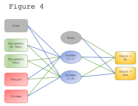
By exploring with different input variables, we can continue to improve the model. Through trial and error, we add household income to the MLP model (Figure 4). 

In Table 4 we see the weights of the new MLP model.

Table 4

Table 5 shows us the prediction classification from the new model that includes household income as an input variable. 

Table 5

From this we can see that simply adding household income as an input, the model now correctly predicts who will churn over 40% of the time. But this still leaves room for improvement, so we continue to work on the MLP model. 

The final MLP model that we explore comes as a result of including all the variables in the data file into an MLP model and then selecting the top 14 input variables based on their normalized importance ratings. 

The resulting MLP model is too complex to include here, but the new prediction classification can be seen in Table 6.

Table 6

The new MLP model accurately predicts those who are likely to churn 54% of the time in the training sample and 56.5% of the time in the testing sample. This is a significant improvement over our first two models. The parameter estimates, along with the input variables included, can be seen in Table 7.

Table 7

The new MLP model is more complex and has a single hidden layer with seven neurons. While this model is significantly more complex, Table 6 shows that it does a better job of predicting who is likely to churn among the telephone company customers. 

Building a neural network: design considerations

When building a neural network, the dimension of the input vector determines the number of neurons in the input layer. In our most recent model there are 14 variables, but because two of the variables are categorical (equipment rental and customer category), we end up with a total of 18 neurons in the input layer plus the bias neuron. Generally, the number of neurons in the hidden layers are chosen as a fraction of those in the input layer. There is a trade-off regarding the number of neurons in the hidden layer:

• Too many neurons produce overtraining.
• Too few neurons affect generalization capabilities. 

Too much in either direction will affect the overall usefulness of the MLP model that is finally developed. 

Deciding how to analyze data 

Machine learning consists of building models based on mathematical algorithms in order to better understand the data. One of the most important steps in understanding the data problem is to decide how the data needs to be analyzed in order to yield the desired results. In our previous review of the telecommunications company example, we used decision tree analysis to develop a prediction model to determine which customer characteristics will help us to predict the customers that are most likely to defect (or churn) and go to one of our competitors. In this paper, we have demonstrated how artificial neural networks are another way to go to develop a useful prediction model. 

The decision tree analysis has its strength in that it identifies those subgroups of customers that are most likely to churn. Those responsible for customer retention can then develop programs designed to reduce churn among those groups most likely to leave.

The artificial neural network model has its strength in that it can be used to develop a forecast model that will predict the number of customers that are likely to churn in the near future. This can be used to predict long-range customer and revenue growth. 

Both decision tree analysis and artificial neural networks are powerful machine-learning algorithms that make it easier to analyze large arrays of data without much programming from the analyst. Both tools still require that the analyst knows which type of algorithm to use for the question being asked and how to interpret the results. 

1. Data source: Telco.sav is an SPSS file that is supplied with the latest versions of the SPSS software.