Editor's note: Doug Berdie is senior business manager at Maritz Research, Edina, Minn.
Since R.A. Fisher’s The Design of Experiments (1935), statisticians have debated the legitimacy and usefulness of tests of statistical significance. Early writers discussed whether these tests should be limited to informing decisions (Neyman, Wald) or are legitimately used for theory-generated hypothesis testing (Pearson, Edgeworth, Yule and other Fisher disciples). Accelerated debate in the 1950s focused on the broader question of whether the tests are relevant at all and in which circumstances they are legitimate. The Significance Test Controversy (Morrison and Henkel, 1970) presents a good synthesis of this mid-20th century debate.
Within applied marketing research, tests of statistical significance have been routinely used over at least the past 40 years, with the results reported in many (if not most) quantitative research reports. Statistical software programs make it easy to conduct such analyses.
Earlier in Quirk’s Marketing Research Review, Baldasare and Mittel (November 1994) and Grapentine (April 2011) discussed some problems related to using tests of statistical significance in marketing research. These include confusion between “statistical significance” and “practical significance” when interpreting test results; selection problems that interfere with sample randomness; and non-response bias that affects data representativeness. These authors point out that survey measurement effects (question order bias, unreliable/invalid question wording, bias from using mixed data collection modes, etc.) cause unknown bias that may outweigh the sampling error that tests of statistical significance are designed to assess.
Three aspects are relevant
Three aspects of testing statistical significance within marketing research are relevant: overall legitimacy of these tests; mathematical legitimacy of these tests; and relative usefulness of these tests.
Some have challenged whether tests of statistical significance are legitimate by arguing that the underlying frequency theory of probability requires assumptions of “infinite hypothetical universes” and other unreasonable assumptions. They conclude that without a sound underlying theory of probability, these tests should not be used. Others have argued the tests are not a valid way of assessing theory-generated hypotheses unless strict experimental designs have been used. Although these debates are intriguing, they are beyond the scope of what follows and will not be discussed further here.
The mathematics underlying tests of statistical significance are less controversial. Hence, we will assume the mathematics are sound.
Today within marketing research, tests of statistical significance are conducted routinely when data from more than one sample or subsample have been obtained. When differences between two or more samples or subsamples are denoted, the question that usually arises is, are those differences statistically significant?
Sophisticated data analysts use tests of statistical significance as one tool for analyzing data. Rarely do they rely on such tests to the exclusion of other analytical techniques when they boil down data to find insights that will facilitate marketing decisions. However, some who analyze marketing research data rely too much on tests of statistical significance. The discussion below hopes to dissuade them from doing so.
Make sound decisions
The objective of applied marketing research is to describe market characteristics so business decisions can be facilitated. The more detailed and precise the information, the easier it is to make sound decisions.
When one places major emphasis on tests of statistical significance, one’s focus becomes yes-no questions such as: Does Sample A differ from Sample B? The answers to such questions are minimally insightful, as they say nothing about the size of a difference that may exist and, without providing that information, decision-making insight is limited.
The following questions exemplify questions that 1) compare one group of people to another group and 2) compare a given group of people over time: How does the preference for Product A differ between women and men? Has the quality of our customer service changed over time?
Many marketing researchers would incorporate tests of statistical significance into their analysis of these questions. Doing so would provide answers such as, “Yes, women and men do differ” (or, “No, we cannot conclude that women and men differ”); and “Yes, our service level has changed” (or, “No, we cannot conclude that our service level has changed”). These conclusions say nothing about the level of preference for Product A or about the size of the customer service improvement/decline. As such, they provide limited insight.
A more useful conclusion to the first question would be, “Women like Product A better than men do.” An even more useful conclusion would be, “About 56 percent of women like Product A compared to about 49 percent of men.” And a much more useful conclusion would be, “Between 52 percent and 60 percent of women like Product A compared to 47 percent to 51 percent of men.”
For the second question, a more useful conclusion would be, “Our service has declined.” An even more useful conclusion would be, “Our service has declined by about 6 percentage points.” And a much more useful conclusion would be, “Our service has declined by 4-8 percentage points.”
The above conclusions facilitate decision-making more than do the simple yes-no conclusions from tests of statistical significance because they tell in which direction the difference is and they provide information as to the actual size of the difference. These more insightful conclusions result from standard statistics used to estimate populations from samples – confidence intervals and confidence levels – which allow us to state the percentage of the time we could expect the results we obtained to fall within a stated data interval.
We see that the above “even more useful” statement (“About 56 percent of women like Product A compared to about 49 percent of men”) contains point estimates of the true values for women and men. To make this statement “much more useful,” we can select a confidence level (any with which we are comfortable) that allows us to statistically derive two confidence intervals (one for women and one for men) showing the percentage of the time the true population values for women and men can be expected to be within those derived confidence intervals. By deciding to use a 90 percent confidence level, we might reach the above, much more useful, conclusion, “Between 52 percent and 60 percent of women like Product A compared to 47 percent to 51 percent of men.”
Nothing magical is required to conclude that more women than men like Product A. (Nor is it necessary, as it is with tests of statistical significance, to create a fictitious null hypothesis and use convoluted logic trying to reject it to reach such a conclusion.) We merely examine the confidence intervals for women and men to see that they contain no points in common. Then we conclude at a 90 percent confidence level that not only do women like Product A more than men do, we can see the actual values associated with both women and men. The answer to the question of whether women and men differ is seen to be of far less interest in itself than is knowing the actual values for women and men.
Applied statistics provides formulas to calculate confidence intervals and their associated confidence levels. These formulas take into account sample size, market size (or, equivalently, population/universe size) being estimated and variation existing within the samples.
Confidence levels and confidence intervals are joined at the hip. As one changes, the other is inversely affected – unless sample size is increased. For example, each of the following two statements could be correct based on a given sample size:
“Between 34 percent and 42 percent of customers (90 percent confidence level) would like our retail stores to be open later.”
“Between 32 percent and 44 percent of customers (95 percent confidence level) would like our retail stores to be open later.”
One can choose any confidence level. By choosing a more stringent level (e.g., 95 percent compared to 90 percent) the confidence interval width will be wider. This is a useful and important because it allows marketing decision makers to decide the relative trade-off between confidence level and confidence interval width.
Statistical literature is replete with formulas for making these calculations. Not always recognized is that selecting the right formula requires considering a host of things including whether one is measuring at the categorical, ordinal or interval level and whether categorical variables being measured are to be reported as binomial or multinomial. In the latter case, one cannot use a simplified formula designed to determine the confidence intervals for yes-no questions if one wishes to determine simultaneously confidence intervals for each of five points in a five-point rating scale.
Two negative consequences
Many analysts, when confronted with piles of computer-generated tables, quickly scan them, earmark “statistically significant” results and ignore other data – based on a dubious assumption that only statistically significant differences between/among groups are important. This approach has two negative consequences. First, it assumes a result shown as statistically significant is worth further consideration – which is not always so. Second, some results that are not statistically significant may well justify further consideration.
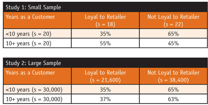
These two consequences result from the heavy influence of sample size on tests of statistical significance. Large enough samples almost always lead to statistically significant results and very small samples rarely do, as shown by the accompanying examples, where the proportionate difference in Study 1 between samples is very large (20 percentage points) yet does not reach a level of statistical significance (at the .05 or even at the .20 probability value), whereas the proportionate difference in Study 2 between samples is very small (only 2 percentage points) – much smaller than the difference between samples in Study 1 – yet does reach a level of statistical significance (at the .05 and even the .01 probability value).

Only designating “significant results” for further attention would ignore the results from Study 1. Yet seasoned research professionals would conclude from Study 1, “That’s a large, 20-point difference. Admittedly, the samples are small (and that’s a factor in why the results are not showing a statistically significant difference) but this is certainly worth investigating further given the marketing implications it may have.”
Similarly, a seasoned researcher would look at the results from Study 2, do a quick marketing cost-to-benefit calculation related to marketing to these the groups differently and, in most cases, ignore this “statistically significant” difference because it is meaningless in a marketing sense.
The best approach is to first scan the data tables to identify differences that are large enough to have a marketing implication and then to consider the confidence intervals around the numbers to see if they are tight enough to justify acting upon them.
The above negative effect is exacerbated by the typical practice of specifying very low probability values (.05, .01) for the test. People do this to reduce Type I error (minimizing the odds of declaring a difference when there is not one). However, the trade-off for minimizing Type I error is maximizing Type II error (increasing the odds of missing a difference that does exist). A focus on minimizing Type I error ensures that even fewer “statistically significant” differences will be found – limiting marketing options brought forward from the research. Surely, this is not helpful to business leaders who seek to identify marketplace opportunities.
Spurious results
By setting a probability value (i.e., a “level of significance”), one accepts that Type I errors will be made. A probability value of .05 dictates that about 5 “significant” results will occur for every 100 tests conducted – even if there are no “real” differences between/among compared samples. Many statistical analysis software packages will compare each table cell to all other cells in that row or, even, all other cells in the table. In a case where responses to a 11-point rating scale are displayed (with each rating point in its own cell) and these responses are shown for each of six subsamples (“brands” in Table 1), if each brand within a row is compared to each other brand in that row, there will be 165 statistical comparisons per table. Because of the probabilities involved, one should expect seven-to-eight spurious (i.e., meaningless) “significant” results to appear in the table. 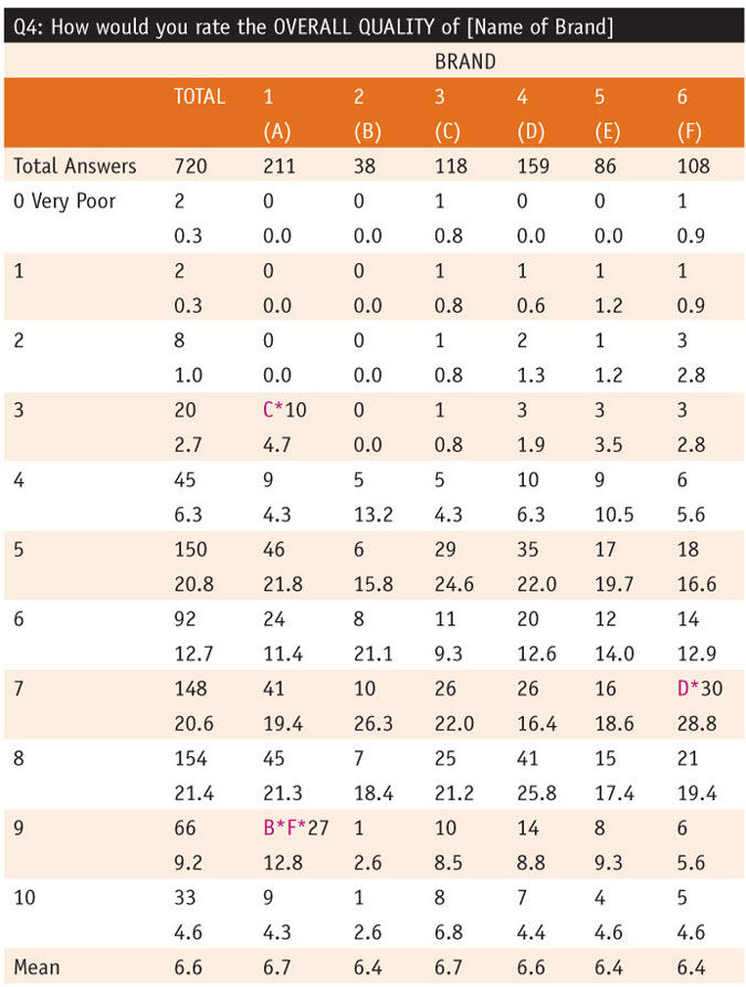
The fact that Table 1 only shows four “significant” differences (highlighted with a red letter and *) suggests all these may be artifacts of Type I error – making it difficult to know which “significant” findings one should pay attention to and which should be ignored.
In the above disguised project, there were 68 ratings questions asked, which means the software made a total of 68 x 165 = 11,220 statistical comparisons. This number of comparisons could be expected to yield about 561 “significant results” even if no real differences exist among any of the six brands being compared. Savvy analysts minimize this problem by limiting the number of analyses to those of real interest. Doing so minimizes the spurious results associated with Type I error and increases the likelihood that revealed statistical differences reflect true underlying themes within the data.
Another problem with conducting tests of statistical significance on each table cell is trying to make sense of seemingly inane results. In Table 1, a “significant” difference exists between the percentage of “7” responses for Brand 6 and Brand 4 – as evidenced in the table by the D* under Brand 6 showing the comparison to Column E that contains Brand 4. Given the 11-point scale, making sense of that “difference” is challenging. And, one wonders, what possible marketing implication it might have. Brand 6 garners a higher percentage of “7” responses (28.8 percent vs. 16.4 percent for Brand 4) but this is offset by lower percentages of both “5” responses and “8” responses for Brand 6. What can that convey of real-world interest? Furthermore, the table shows no “statistically significant” difference between the means of those brands so, if one were to play the significance game, on the one hand one would see a “significant difference,” while on the other hand one would not. Over-application of tests of statistical significance does not lead to greater insight – it leads to interpretative chaos.
Indicates a misunderstanding
Test-of-statistical-significance advocates assert that lower probability levels indicate more meaningful differences between/among groups. Yet to claim a test result of .001 is more significant than a result of .05 indicates a misunderstanding of how probability values apply to tests of statistical significance and leads to confusion over practical versus statistical significance. A lower probability value attests to the confidence one can have that there is a difference between/among groups. It says nothing about whether the difference itself is meaningful in an applied marketing situation. However, due to linguistic confusion, when users assert they have found a “highly significant” finding (e.g., p<.001), this assertion tends to convey that the difference is a “really important” one. However, only if the magnitude of the difference has marketing implications should one be concerned about its statistical characteristics.
Why are they still used extensively?
If tests of statistical significance yield less insightful interpretations than techniques for estimation, how did their use become prevalent and why are they still used extensively? One might speculate as to reasons.
First, professors who teach tests of statistical significance (in business and social sciences statistics courses) typically are not engaged in applied marketing/social research themselves and conduct more theoretical research. Tests of statistical significance may be more relevant to academics because their interest is in testing hypotheses to see if the theories from which they derive find support from the tests.
Second, the results from tests of statistical significance provide an easy tool that allows researchers to make quick decisions without having to spend time digging into the data and working with decision makers to understand all the ramifications of the results on impending decisions. It is easier to conclude that the test shows no significant difference, and therefore you should not market deodorant to women differently than you do to men than it is to say that the small sample size we used may be masking an important difference regarding how women and men react to deodorant marketing and, given the size of this market and dollar implications of the decision we must make, it may be wise to do some follow-up research before finalizing a segmentation go-no go decision.
Third, marketing research has its own set of esoteric terms and practices that can be used to enhance the credibility of its work. Tests of statistical significance fall into this category.
Fourth, marketing researchers who rely extensively on test-of-statistical-significance results are, in a sense, able to evade responsibility for making tough decisions. It is difficult to argue with someone who staunchly cites criteria that many colleagues share and support.
Fifth, most statistical analysis software packages contain programming that facilitates calculating tests of statistical significance. This makes it easy for applied marketing researchers to either program these tests themselves or request that others, “Run some crosstab tables and specify t-tests [or chi-square tests or some other type of statistical test] at the .05 level.” However, merely having the capability to run a test is no guarantee it is legitimate or insightful to do so.
Little help
Tests of statistical significance used to compare two or more groups yield yes-or-no answers. They tell us that, yes, these groups likely differ from each other or no, we cannot conclude these groups differ from each other. When testing theory-generated hypotheses for the purpose of seeing if a theory is valid, these yes-or-no answers may be useful. However, when practical business decisions need to be made, merely knowing that one group differs from another is of little help without some estimate as to the size of the difference. Hence, placing primary focus on tests of statistical significance in applied marketing research is not advisable.
Clearly, tests of statistical significance are overused and often abused within applied marketing research. However, before marketing researchers will adopt more insightful alternatives such as increased use of confidence intervals and confidence levels, these alternatives need to be emphasized in business and social sciences statistics courses. And, software packages for analyzing research data need to include options that allow users to easily and accurately run these analyses. One can hope these educational and accessibility changes occur quickly.
The additional insight provided by using statistics of estimation instead of tests of statistical significance, and the more straightforward means of interpreting results from these tools, will enhance the use of marketing research data and help overcome a persistent criticism by business decision makers that marketing research data do not result in the level of insight desired to make sound business decisions.