Editor's note: Rajan Sambandam is chief research officer at TRC Market Research, Fort Washington, Pa.
What is the right sample size for a conjoint analysis study? It’s a simple, ubiquitous question that doesn’t seem to have an easy answer. Bryan Orme (2010), president of Sawtooth Software, the maker of the most widely-used software for conjoint analysis, lists a variety of questions that could affect the answer. He recommends some general guidelines (such as having at least 300 respondents when possible) but does not provide a more specific answer. Given that, is it possible to come up with a general recommendation that can be easily applied by practitioners? Specifically, is it possible to develop a simple, practical recommendation that can be applied before knowing any details about the study? We think it is.
Let’s start with what we normally do when estimating appropriate sample size in market research surveys. There are two common approaches to sample size estimation – based on a single number or based on the difference between numbers.
For a single number from a survey, we are usually interested in understanding the associated precision. Conventional margin of error calculations can estimate the error bound around a single proportion (the calculation for proportions is easier than that for means and hence more often used). Since a sample of size 400 has about +/- 5 percent margin of error, we can be confident that it can keep the error below +/- 5 percent. Our error tolerance and budget will decide if this is an appropriate sample size for a study.
Alternatively, we can think about the sample size that is likely to yield a significant difference between two numbers (say, proportions). An independent samples t-test is commonly used to understand if two proportions are different. As before, it can be reversed to determine the sample size needed for a given difference to be statistically significant. For example, to detect a difference of 7 percentage points, a sample size of about 400 is needed.
In practice, samples in the n = 400 range are often taken as an acceptable default, as error reduction begins diminishing beyond that. And of course, if subgroup analyses are required, overall sample size may need to be adjusted to compensate. The great advantage here is that these calculations are made without needing to consider the number or type of questions in a survey. So, sample size decisions can be usefully made ahead of time, rather than waiting for questionnaire finalization.
But conjoint analysis is not the same as asking simple, direct scaled questions in a survey. Let’s consider what is different about the conjoint process, how it impacts sample size and if there’s a way to determine it ahead of time.
Sample size in conjoint
For the purpose of this discussion let’s assume we are talking about discrete choice, the most widely-used type of conjoint analysis. Respondents are repeatedly shown a few (say, three to five) products on a screen (described on multiple attributes) and asked to choose the one they prefer. A typical conjoint exercise is considerably different from a simple, direct, scaled question. On each screen a respondent has to consider several attributes, usually involving a trade-off between benefits and costs and has to provide a response (and repeat several times). Many factors can vary between studies, such as the number of attributes and levels per attribute, number of products displayed per screen, number of screens per study and sample size. In developing the design for a study, all these factors have to be taken into account. How does sample size fit into this?
Traditionally conjoint designs (once finalized) are tested to estimate the standard errors that are likely to occur with the utility scores (which are the primary output metric). A standard convention is to ensure that all utility scores have standard errors of .05 or less (which translates to about +/- 10 percent error bound around utility scores). The test determines what sample size will provide the target standard error values. Beyond the fact that this can only be done with software when the design is finalized (and hence quite late) there are a couple of other problems. One is that the test is only an approximation and the other is that the utility scores are not the primary output metric of interest.
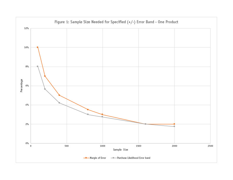
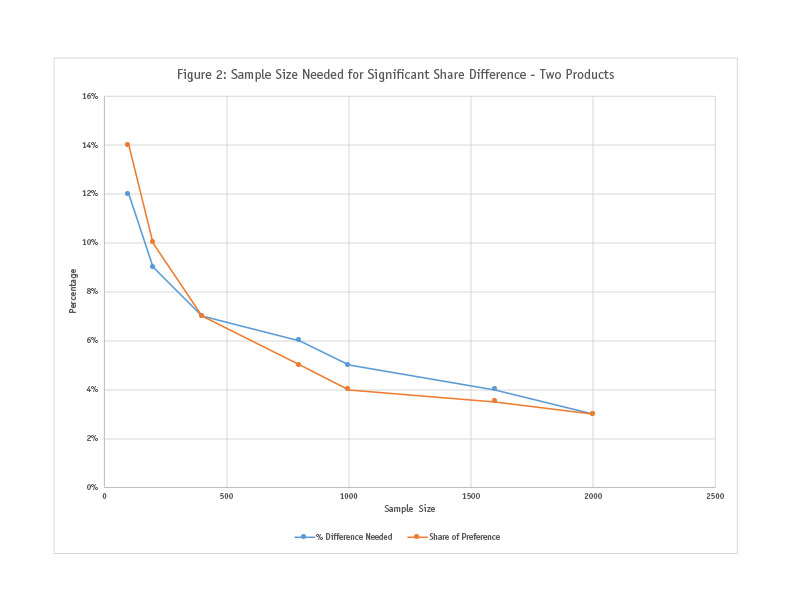
The actual output metrics that are of practical interest are utilities of attribute levels transformed into shares of products, specifically purchase likelihood scores (in the case of single product simulations) and shares of preference (in the case of multiple products). Products created in the conjoint simulator are often evaluated using these metrics to determine appropriate market actions. In the case of purchase likelihood scores, the manager may be interested in the uncertainty (error band) surrounding the score, while in the case of share of preference the interest may be in determining whether the shares of two products are significantly different.
This is, of course, very similar to the situation in regular surveys when determining sample size. So, the question is whether the same calculations used to determine sample size in regular surveys can be applied here. One way to answer this question is to do so empirically. That is, we can take an actual conjoint study, compute purchase likelihood, share of preference values and related error bounds, which can then be compared to the corresponding general survey calculations. Repeating this process over a variety of studies will allow us to generate enough data to determine if the sample size calculations applied to general survey data are applicable to conjoint results.
We tested 10 studies ranging in size from two to nine attributes, with two to 10 levels per attribute. The number of respondents per study varied from 402 to 2,552. Since studies with larger sample sizes can also be tested with randomly chosen subsets of data, we ultimately had 29 data points to study. For purchase likelihood, we developed a distribution of margin of error scores for each study, to identify the maximum error. For share of preference, we created a series of two product simulations (with shares in the 40-60 percent range) and tested the difference in share required for statistical significance at various sample sizes. (Technical note: This is the classical t-test rather than the Bayesian version where results may differ).
Charted results are shown in Figures 1 and 2.

When regression analysis is conducted predicting purchase likelihood and share of preference needed for significant difference, we find excellent models (with near perfect R2 values). In both cases, the beta weight is about 0.80, implying that using conventional sample size calculations is a slightly more conservative approach.
The close correspondence between the sample size calculations for regular surveys and for conjoint shares makes sense given that the only variables used in these tests are the proportions (shares) and standard errors. Simply put, if a set of proportions and standard errors are available, their origins may not matter, only the outcome.
This raises a couple of questions.
Question 1: What about complexity? Earlier we said that the complexity of conjoint questions makes them different from direct survey questions. Hence even if sample size calculations from regular surveys apply to conjoint results, would they not vary based on study complexity? For example, would more-complex studies require larger sample sizes? Study complexity can be based on a variety of variables such as number of attributes, levels, concepts per screen, etc. We have not been able to test all of them, but by varying the number of attributes (< five and seven-to-nine) we found no difference (using four data points in each group). Further, in Figure 2 (which has 29 data points), the average scores at each sample size are displayed but the actual variation is quite minor, indicating that the study complexity does not have much of an impact on the sample size calculations. While we cannot say definitively that complexity does not impact sample size consideration, for most practical conjoint studies it would appear that complexity should not be a factor. But when studies have abnormalities in design (say, 12 levels for an attribute), it might be useful to consider increasing the sample size.
Question 2: Can I use fewer choice tasks? This is a common question that comes up as the design is being finalized and is generally triggered by the prospect of an overly long questionnaire. The subtext here is that this is to be done without increasing sample size for the study. We analyzed two studies by comparing results from the full set of choice tasks with that from a half set of randomly chosen choice tasks. As expected, margin of error increases (for purchase likelihood) while the ability to detect significant difference decreases (for share of preference). So there is a clear sacrifice that is made when fewer choice tasks are used.
Johnson and Orme (1996), show that the number of choice tasks and sample size can be traded off. Orme (2010) considers two common forms of survey error and suggests that sampling error is based on sample size and measurement error is based (mainly) on number of choice tasks. Hence the implication is that total survey error can be managed by trading off between the two types of error. For practical purposes, one way to think about this is in terms of sample availability. When sample is cheap and plentiful (e.g., B2C), perhaps a compromise can be made in terms of fewer choice tasks and more sample when questionnaires get too long. When sample is expensive and limited (e.g., B2B), the opposite approach may work better.
Can be easily calculated
Conjoint studies go through various stages of design and iteration. How do we determine appropriate sample size before we know anything at all about the design? The simplest recommendation based on outcome metrics of practical interest is to use conventional margin of error and significance testing calculations as guidelines. These are well-known and widely-used heuristics that can be easily calculated and appear to be somewhat conservative. If there is a sense that the study will have abnormal complexity, it may be prudent to increase the sample size beyond these guidelines.
References
Johnson, Richard and Orme, Bryan (1996), How many questions should you ask in choice-based conjoint studies?, Sawtooth Software Research Paper Series.
Orme, Bryan (2010), Getting Started with Conjoint Analysis: Strategies for Product Design and Pricing Research, Second Edition, Research Publishers LLC.