Conjoint analysis has a long history as a powerful method for developing the best set of features for products and services. Its strengths in creating the best mix of elements in communications, though, are less well-known. Its newest application, for improving Web sites, while in its beginnings, already is showing great power and promise. This method allows us to see the value of hundreds or even thousands of alternative communications, all in a single test.
We will first briefly explain conjoint and how it works and then go on to the specific applications.
Advantages immediately apparent
Conjoint was hailed as one the greatest advances in determining what people really wanted when it first appeared somewhere around 1975 – and for many years following. Several advantages were immediately apparent. First, it asked people to trade-off valuable features vs. each other, rather than just rating features in isolation.
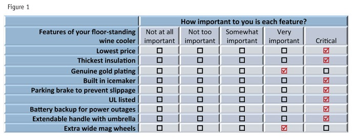
The way people use rating scales posed (and still poses) one of the thorniest problems in learning what is actually important to them in a product or service. As we can see by looking at the importance ratings of a fictional respondent in Figure 1, it is easy to rate everything as highly important – and that is what people generally do when asked outright to rate individual features of a product or service.

Conjoint moves well beyond this by showing features in the context of the overall product – at least in its full-profile version. Full-profile simply means that study participants respond to a whole product or service, typ-ically described as a set of features or attributes. (There are other variants of conjoint, including partial-profile and adaptive – but in recent years these seem to have had relatively little use.) Conjoint shows people a number of product descriptions or profiles and asks either for ratings (or more rarely) rankings of each.
Let’s move on to a venerable example dating to the 1990s, the industrial macerator. This is a strictly fictional machine but it does have a marked resemblance to a real one. Our ersatz client, Ace, nearly owns this market, with an 81 percent share. This will make conjoint a good choice for figuring out how to improve its machines. (We will talk briefly about using conjoint vs. using discrete choice modeling later.)
Let’s discuss the different features and the ways in which they can vary. The different variations of a feature, as a reminder, are called its levels. Here are some facts about the machines, and then the levels that our client wants to test.
Price: These machines can cost between $46 and $88 million. Ace, however, considers itself the quality leader and so will not sell any machine for less than $52 million. It will not bother testing the lower prices used by its main competitors, Puny Industries and Insignificant Corp.
Sparge pipes: They can have two, four or six pipes. Ace has just patented an eight-pipe “professional” design, which it wants to introduce and hopes will be the next big thing in macerators.
Extra features: These machines also can have three to 17 high-speed stridulators.
Colors: They come in a wide range of attractive shades: black, brown, olive drab and pink.
Here is what Ace decided to test:
Price: four levels – $52 million, $60 million, $74 million and $88 million.
Sparge pipes: four levels – two, four, six and eight.
Stridulators: four levels – three, seven, 12, 17.
Color: four levels – black, brown, olive drab and pink.
With just these features and variations, there are 256 possible configurations (4 x 4 x 4 x 4). Conjoint analysis allows us to use very carefully constructed subsets of these, based on an experimental design. Experimental designs enable us to vary many attributes at the same time and still measure the effects of changing each one separately. We will need to show just 16 carefully configured product profiles to determine the worths of all 256 possibilities.
Here is a sample of a conjoint screen (or card, as they are sometimes still called) that a respondent would see and evaluate.
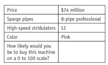
If the industrial macerator had the features you see below, how likely would you be to buy it? Please think of just this macerator and nothing else you may have seen. Assume you really need a macerator. Please use a 0% to 100% scale. You may use 0%, 100% or any number in between, depending on how likely you are to buy a machine like this.
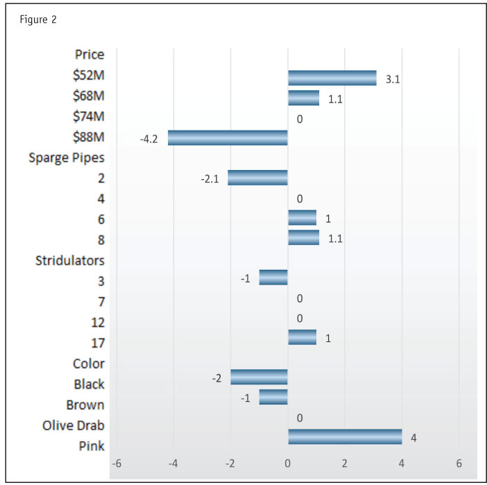
With everything analyzed, a summary of the values or utilities of the different attribute levels emerges. These utilities clearly show what is most desirable.
Figure 2 shows how the utilities look. Reviewing this chart, we can see that the marketing department was right and the unit really needed to be a new color. Also, we see that dropping the price to the lowest level is what the market wants, and that the eight-sparge-pipe “pro model” is not too likely to revolutionize the industry.
When questions arise about how much good any change will do in the marketplace, conjoint analysis must make assumptions about how utility values become market share. This has been a historical weakness of conjoint analysis: It is wonderful at showing the relative values of different features – and variations in those features – but it does not do well enough at showing effects in the marketplace. For that we need to use discrete choice modeling (DCM) or, as it is sometimes called, choice-based conjoint.
Go directly to behavior
Fortunately, when we are dealing with messages, we are trying to pick the best alternative – so the issue of how utilities become marketplace behavior is largely sidelined. And with Web sites, even though we still use a con-joint-style approach, we go directly to behavior, such as clicks or stickiness (how long a person stays on the page or site). Because we are interested in what generates the most behavior, we will again steer clear of the problem of estimating market shares. And again, anywhere we use conjoint, we get the equivalent of testing hundreds or even thousands of alternative message configurations, all in one simple test.
Some disagreement exists about the differences between discrete choice modeling (DCM) and conjoint. For our purposes, if you are using rating scales as part of a trade-off exercise, then that is conjoint. If you are showing products side by side and asking people to make choices, then that is DCM. Showing people one thing at a time most often means you are using conjoint analysis. That is why we are calling the extension of this method to testing Web sites “conjoint,” even though we are measuring behavior there.
Our first example is a direct mail piece, one of those insurance offers we all look forward so much to receiving. It's an early, fictionalized instance of conjoint being applied to develop the best mix of elements in a message. Because these insurance offers are designed to work with very low level of responses (often under 1 percent), even a fractional improvement can make a vast difference. If you move from 0.8 percent to 1.0 percent response, you have increased your sales by 25 percent (that is, this is the 0.2 percent increase divided by the 0.8 percent base rate).
There are two components to this offering: the envelope and the letter. Figure 3 shows a disguised idea of what was tested. There are six features or attributes that get varied. Counting the variations or levels we get to how many cards, or message profiles, we will need to show. The more attributes and the more variations per attribute, the more cards or profiles we will need.
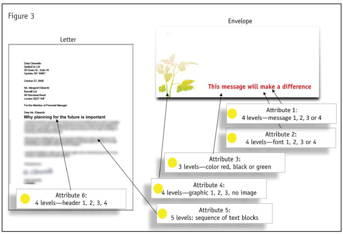
Specifically here, we have four attributes each with four levels; one attribute with three levels; and one with five levels. There is a formula for how many cards this will require. First, we take the number of attributes times the number of levels. Specifically, we have (4 x 4) + (1 x 3) + (1 x 5); that comes to 16 + 3 + 5 or 24. Then we subtract out the total count of attributes, which is 6. That gives us 18. We need to add back two more so that we can measure error and we can estimate a term called the constant.
We have just measured degrees of freedom (which some of you may recall with dismay from your statistics classes) and made sure that we have at least one card for each degree of freedom.
We finally used 24 cards and showed each person eight of them. That is, everybody saw just one-third of the total cards. So, in effect, everybody counted for just one-third of a complete set of responses, or perhaps, one-third of a whole respondent.
As an aside, when we did this many years ago, it required us to triple our sample. Now though, thanks to the nearly magical-seeming properties of hierarchical Bayesian analysis, we actually can get much more per respond-ent. We might possibly even get away with no increase in sample, although experience has shown that when dividing the total task into three pieces, boosting the sample by 50 percent is safer.
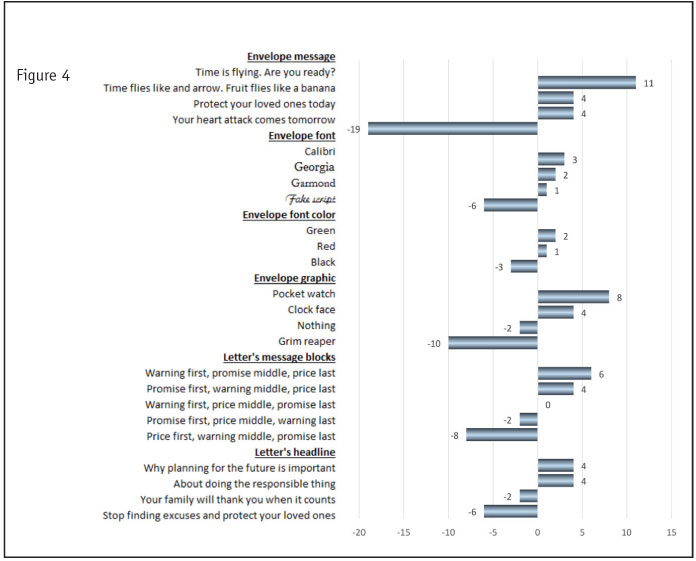
Back to our main story, here is the way the utilities looked (in Figure 4). Here we have tested the equivalent of 4 x 4 x 3 x 4 x 5 x 4 or some 3,840 alternative combinations of message elements, and have found the apparent best one:
• Time is flying. Are you ready?
• Calibri font on envelope
• Green ink on envelope
• Letter: Warning first, promise next, message last
• Letter: Why planning for the future is important
In this instance, there was a direct way to test whether this combination worked, as the design the client was using was one of the combinations with lower total utility. And by switching, the client actually improved its response rate by some 25 percent, just reaching the magic 1 percent acceptance mark. So this was an early success story.
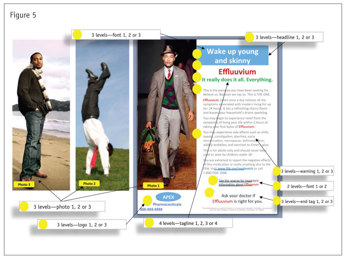
Our second example comes from a test of a print advertisement. The same principles hold as in the test of the direct mail campaign. Figure 5 shows our slightly fictionalized ad and the elements varied in it.
Here we would have an immense number of possible variations. That is, we would have: 3 x 3 x 3 x 3 x 2 x 3 x 3 x 3 or 4,374 possible ways of combining these elements.
We can determine the value all of them with 18 experimentally-designed combinations.
How would this look to a study participant? In Figure 6 we see how one profile in the test would look, using another combination of elements based on the experimental design.
This was an online test, with each person exposed to eight alternative combinations or profiles out of a total of 24 used for the test. Accompanying the Figure 6 test were these instructions:
Assuming this was the only message about this product, how likely would you be to prescribe the product to a typical patient with atypical depression? Please think of just this message and use the 0 to 100 scale where 0 means “absolutely unlikely” and 100 means “absolutely likely.” You can use any number from 0 to 100, but try not to rate any two messages the same, as they are all different.

The outcome
Based on this test, the client was able to determine easily which of the over 4,300 possible combinations generated the most interest. This was done with a chart showing the basic utilities, just as we did in the last example. This study, however, involved another interesting issue, which we could call the presence of a HIPPO. A HIPPO is simply the highest paid person’s opinion. The Big Boss really wanted to know how a few of his favorite ideas played out against the best combination.
This seemed to call for a simulator, similar to a market simulator, but in this case with the overall rating as the outcome. Figure 7 gives an idea of how the simulator looked.
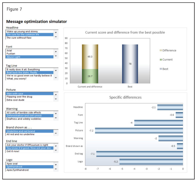
As we can see, the Big Boss’ favorite is roughly one-third as well received as the best possible combination. This led to the truly difficult part of the study: The researchers in the organization would spend the next week trying to figure out exactly how to convey this information.
Works well with Web sites
This approach works extremely well with Web sites, as testing can take place using the actual behavior of visitors to the site, rather than asking people to provide ratings. This is how it works:
• Just as for print, the list of features to be varied is created.
• The variations are put into an experimental design.
• Alternative executions are made up.
• When people visit the site, they are randomly assigned to one of the alternatives.
• Clicks and/or stickiness (amount of time a person spends on the page) get measured.
• With extreme values removed or rolled back to more reasonable levels, we solve for the target variable (clicks or stickiness).
Getting rid of extreme values is important – a person may appear to stay on a Web page for a long time for many reasons (answering the phone, doing several things at once, putting out a kitchen fire and so on). Also, vanishingly small times suggest a mistaken click on the site – and so likely are not a reflection of interest levels.
In Figure 8, we see how a fictionalized Web page with five elements being varied looks. (The superimposed numbers are there just for our reference – they would not appear in the test.)
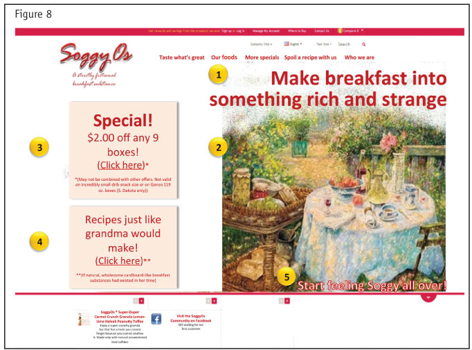
We in fact have five elements, each varied in four ways. This comes to some 1,024 alternative combinations of the varied elements (or 4 x 4 x 4 x 4 x 4). To test the value of all possible combinations, we needed to develop and test 20 alternatives in an experimental design to get accurate measurements. (This again is based on the calculation of how many degrees of freedom we have in this design – namely 5 x 4 minus 5, then plus 2 to measure error and the constant. We used the next even multiple of 4 above this, or 20.)
Needing 20 alternatives leads to a caution: You need a fairly well-visited Web site to do behavior-based testing of this type. If each person sees just one of those alternatives, then that person is just 1/20 of a complete set – or that person counts as just 1/20 of a complete respondent.
Sticking with a fairly slender requirement of 125 complete respondents, we would need 2,500 visitors to complete one test. So you do need a relatively busy site to do this kind of testing.
This may seem to demand a great deal of traffic to get an answer – and if so, then nothing prevents you from testing the elements for a Web site in the same way as you would test a print advertisement. That is, you would recruit people to a survey and then show each person a number of alternative site designs. The live test has the advantage of measuring actual marketplace behavior – and presumably among people who are interested in the product or service. In the survey’s favor, if we questioned people, we also could ask other questions about who the respondents are, their usage of other products, and so on.
Find the best mix of elements
We have outlined some of the useful ways in which conjoint analysis can find the best mix of elements in communications. No other method gives you nearly the same ability to determine the value of so many alternatives at one time – hundreds or even thousands in a single test.
We have just touched on the complexities that underlie this (which we suspect you will forgive). Fortunately, the area in which conjoint has received the most criticism – uncertainty about the way in which the utilities it produces actually become choices in the real world – does not matter as much when you are trying to pick the best combination of message elements. Because of this, conjoint stands as particularly well-suited toward testing communications of many types.
REFERENCES/ADDITIONAL READING
Gelman, A, et al. (2002). Bayesian Data Analysis. (Boca Raton, Fla.: CRC Press). This book has a thorough discussion of hierarchical Bayesian modeling from a more theoretical standpoint. It requires that you read a good number of equations but the text is relatively readable.
Lyon, D. (2000), “Pricing research,” in Chakrapunti, C. (ed.), Marketing Research: State of the Art Perspectives, pp. 551-582 (Chicago: American Marketing Association). This discusses strengths and weaknesses of conjoint with specific reference to pricing.
Morwitz, V. (2001), “Methods for forecasting from intentions data,” in Armstrong, J.S., Principles of Forecasting, pp. 33-57 (New York: Springer). This article outlines approaches to using ratings data in making forecasts and points to the lack of agreement about acceptable methods.
Train, K. (2009). Discrete Choice Modeling with Simulation. (New York: Cambridge University Press). The second edition of a standard text on discrete choice modeling, with a thorough explanation of the mechanics of these analyses. Numerous equations but still readable.
Wittink, D. (2001), “Forecasting with conjoint analysis,” in Armstrong, J.S., Principles of Forecasting, pp. 147-169 (New York: Spring-er). This discusses some more successful applications of conjoint and traces its development and history.