Editor's note: Steven Struhl is principal at SMS Research Analysis, Philadelphia.
Just when we were starting to feel comfortable with our state of confusion about statistics, another remarkably powerful set of analytical methods with new rules has appeared. They are variously called Bayes nets, Bayesian networks, Bayesian belief networks and probabilistic structural equations – and generally, computational tools to model uncertainty.
Importantly for us, they work in many practical applications and often work better than other methods.
Bayes nets can quickly focus on important variables, show how variables are connected, what the importances of variables are with terrific accuracy and build models with strong predictive power. They even bring us closer to what may approximate the Holy Grail in research: showing clear linkages between survey data and market share.
Bayes nets have many remarkable capabilities and, inevitably and unfortunately, some new terminology. We will need two installments to cover their basic functions and to give some examples of how they work. In this month’s article we cover some background, including what Bayes nets do and what makes a Bayes net Bayesian. We will touch on some of the ground rules and then discuss the central concept of conditional probability.
To show how conditional probability can solve problems that really elude us intuitively, we will see how reliable a witness actually is when he says he saw an accident. Then we will solve the famous (or infamous) Monty Hall Let’s Make a Deal problem in which you will get to decide whether to stick with the door you chose or switch to a different one. The answers will surprise you!
We will round out this installment with some more basics, discussing networks and the value of information, and finally will compare networks with regressions.
In the next installment we will get to the examples, showing the remarkable powers of these networks in practical applications. We will first show how a network automatically found logical and informative patterns of relationships in questions from a typical big, messy questionnaire. We will conclude with a network linking questionnaire questions to market share with over 70 percent correct prediction levels. This example strongly suggests that Bayes nets may well be the next new thing, greatly expanding our ability to understand variables and their effects.
Have proven themselves
Networks are new to research and the social sciences but they have they have proven themselves in many other fields. They have served for years as reliable and valuable additions to the analytical armamentarium. So the bugs have been worked out and there are a host of highly useful applications. Work that was directly applicable to the development of Bayes nets goes back at least to the 1940s. Judea Pearl’s Probabilistic Reasoning in Intelligent Systems: Networks of Plausible Inference, which discusses principles that underlie these nets, dates back to 1988.
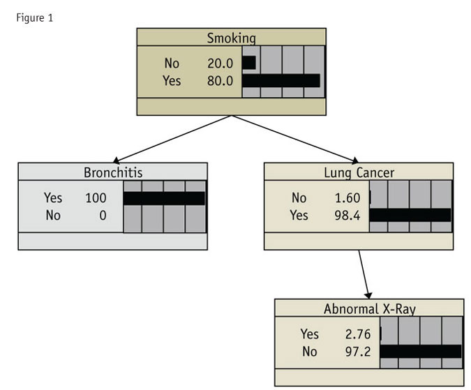
A network can be simple, like the example in Figure 1, which shows the relationship of cancer, bronchitis and abnormal X-rays. (Set as it is, it shows what we can expect in the other areas if a person has bronchitis.) Networks can become so complex that reading them becomes quite difficult.

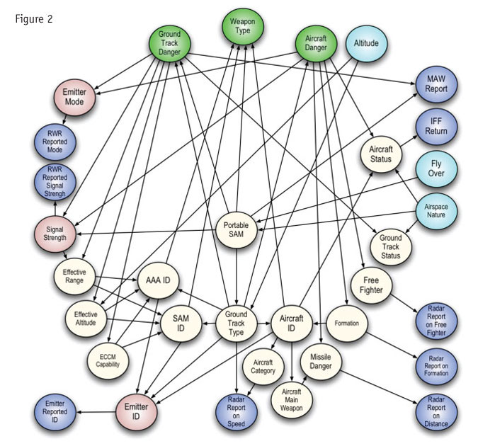
Figure 2 is one that is nearly unintelligible, but that still works. It has a genuinely serious application, namely deciding whether to launch a missle. This at least should give us some confidence that these networks are in fact (and not just in metaphor) battle-tested.
Bayes nets are a powerful and flexible set of approaches that can solve many problems. The variety of uses can range from brainstorming to highly sophisticated modeling and forecasting systems. Here are some applications:
- automatically finding meaningful patterns and connections among variables;
- getting accurate measures of variable strengths (for drivers analysis);
- screening large numbers of variables quickly (for data mining);
- linking questionnaire data to data from the outside world, such as market share;
- developing models of cause and effect (in the right circumstances); and
- incorporating expert judgment into data-driven models.
Everything Bayesian refers back to the work of the Rev. Thomas Bayes, who lived an apparently quiet life in Tunbridge Wells, England, in the 18th century. He published two books in the 1730s, but never the “Bayes’ theorem” that bears his name.
Bayes’ formulation itself is simple. We should add that he never called it a theorem and that any reasonably literate person could easily understand it in its entirety, aside from what one writer1 astutely calls the “goggle-making” formulation often used to represent it. Starting from Bayes’ straightforward assertion and arriving at many of the types of analyses that bear his name likely would have caused the good reverend to take on a strange hue.
We can formulate Bayes’ idea in a variety of ways. Let’s start with this more practical formulation:
We start with “prior” (existing) beliefs and we can update or modify these by using information on likelihoods which we get from data we observe. Adding this information gives us a new and more accurate “posterior” estimate. From this posterior estimate, we draw conclusions.
That’s really all there is to it.
However, it is usual to encounter this formulation, which can indeed make many readers’ eyes goggle:
P(Bi|A) = P(A|Bi)P(Bi)/∑i{P(Bi)P(A|Bi)}
Yet this notation simply reflects what we said in the modest paragraph above.
The Bayesian approach also includes the idea of conditional probability. This phrase appears prominently in many discussions. However, a probability that is conditional on the data is no more than what we just described: an estimate of probability that is revised based on including information from data into some prior estimate or belief.
The ground rules for networks
Diagrams of variables are key. A Bayes net calculates relationships among variables and shows how they fit together. A diagram of how variables relate to each other therefore is integral. Somewhat more formally, these networks are based on graph theory and on probability theory – so grasping their workings requires both a diagram and calculations with it.
Looking at a network, you will see a familiar type of diagram, if you have experience with structural equation models (SEMs) or with partial least squares (PLS) regression path models. Variables are connected with arrows, or arcs, showing pathways between them and these lead to target variables.
Directions are important. In a Bayes net, there must be directions between the variables and there cannot be any circular or cyclic pathways where a variable points back to itself. This is why these networks are sometimes called directed acyclic diagrams – or, as you may encounter in the literature, DAGs.
The arrows or arcs have a specific meaning in these diagrams. However, this is largely intuitive. A variable at the start of an arrow leads to another variable and in certain conditions we even can say that the starting variable causes the variable at the end. Arrows can lead to or from a target variable.
Terms and phrases: It’s all in the family. There is of course some terminology to learn (Figure 3).
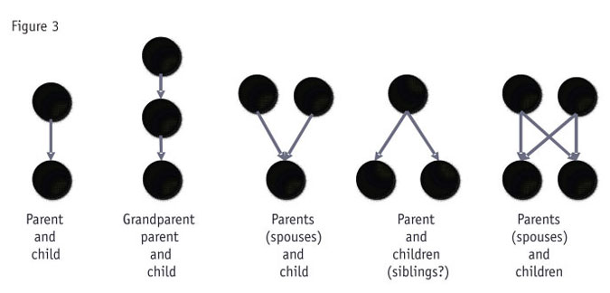
Fortunately, much of this too is largely intuitive and rather uncharacteristically warm-and-fuzzy for statistics.
- The variable at the start of an arrow is called a parent.
- The variable at the end is called a child of the parent.
- Children can have several parents and parents can have several children.
- If there are two or more parents, they are called spouses.
- A parent of a parent is a grandparent and so on.
- Variables are dependent only if they are directly connected. Children and parents are dependent on each other. Children are independent of grandparents and other variables further away.
Whether variables are dependent on each other becomes important when screening variables for inclusion in a model. One powerful screening technique is to include only those variables that are dependent on the target variable (its parents and children) and the other parents of any children. Closely-connected variables have stronger effects, so this quickly eliminates less-important variables where there are many – as in data mining applications. This set of variables has a name also: the Markov blanket. (How Mr. Markov enters consideration is something to talk about another time.)
Related to whether variables are dependent, there is another item of terminology that you may encounter. The variables have “edges” that go with the arrows. The edge of a child node points toward a parent node.
Everything is connected: Changes move through the whole network. Regardless of dependencies, all variables in a network change when one changes. This sometimes is described as “information propagating through the network.” The whole network is connected. And indeed, as we will soon see, understanding networks as conveying information is critical to their practical applications.
This connectedness throughout the network also makes estimates of variables’ importances much more powerful and accurate than those we can get from regression-based models. Using regressions, we need to assume that when we change one variable, all others remain constant. This can happen if we set up an experiment but with real-world data, this is hardly ever the case.
However, with a Bayes net, any effect we see takes into account all the connections to all the other variables. We are considering the entire system when we measure any effects.
Network-building ranges from simple to complex. As follows, when we are modeling relationships among variables, our choices in how the network gets put together are of prime importance. There are many, many ways to get a network assembled automatically. At their simplest, there are methods in which all variables get fit directly to the target variable as well as possible. This is very much like a regression where all variables are put in without screening to see which ones belong.
Networks at their most complex result from countless attempts to fit the data – finding how variables best fit together to predict or explain the target variable. These methods use sophisticated tests to ensure that the network does not seize upon a connection that is good “locally” (where a variable is being added) but not good for the overall network.
Did somebody say we can figure out causality? Finally, we did mention that we can, at times, see whether one variable actually causes another. The idea of finding causality in networks is quite intriguing. However, when we build a network from the data we typically use, we often discover that some arrows work as well in either direction. These directions are “equivalencies” and we must decide how the arrows point.
Only if an arrow must point in one direction can we say that one variable causes another. There are tests that determine this. Unfortunately, rarely does the data we find in surveys have completely definite directions among the variables.
Conditional probabilities
Bayes nets involve conditional probabilities, which in practical terms means how the distribution of values in each variable fits with the distribution of values in other variables.
More practically, networks can solve problems quickly that are difficult or elusive to solve using other methods. The workings of conditional probability can be difficult to envision, so hold on and we will try two small examples: the yellow taxi-white taxi problem and the “three-door” Monty Hall problem.
Yellow taxi-white taxi
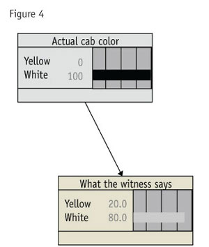
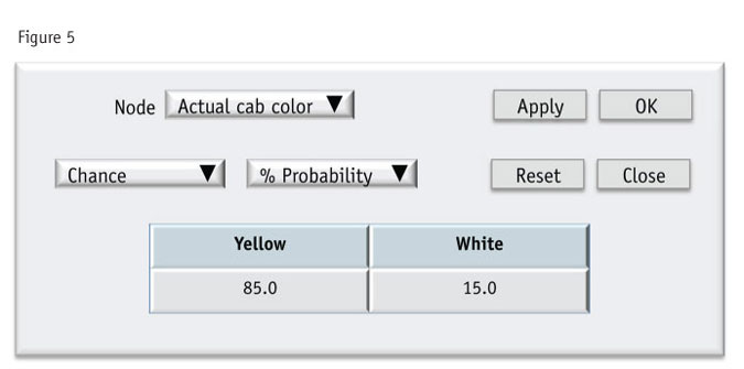
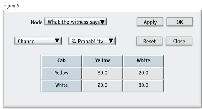
There is an accident involving a taxicab. A witness reports that the cab involved was white. In this city, 85 percent of cabs are yellow and 15 percent are white. The police actually test the witness out on a street corner and find that he is 80 percent accurate at getting the cab’s color.
What are the odds that the cab actually was white? We can solve this with a simple Bayes net2.
Setting up the taxicab problem is simple. Recall that we can make a network ourselves by linking up variables, just as we can create a network from a data file. Here we will form the network by linking two events: the color of the cab and what the witness reports as the color. Each event is called a node.
We understand that the actual color of the cab leads to what the witness reports as its color so we will draw a small network with the color of the cab leading to what the witness reports (Figure 4).
First we set up the node showing the odds of a taxicab being yellow (Figure 5). Next we set up the second node showing the odds of the witness being right about each type of cab (Figure 6).
Now what happens when the witness says he definitely saw a white cab? In the diagram, we will change the value of “What the witness says” to 100 percent for white. Since cab color and what the witness says are linked (as we showed in the diagram), if we change the value of one node, the other will change along with it. So even though the arrow points from cab to witness, if we change the value for “witness” we will see the change flow back to the likelihood of the cab being a given color.
This is a basic property of networks. All variables are connected so that all change when any one changes. This keeps their defined “joint probabilities” in line.
Now for the surprising answer. The bars to the right in Figure 7 allow us to manipulate the levels for the witness or the cab. We set “white” in the witness node to be 100 percent. That is, this corresponds to the witness saying the cab is white. The node takes on a gray color to signal that we have changed it.
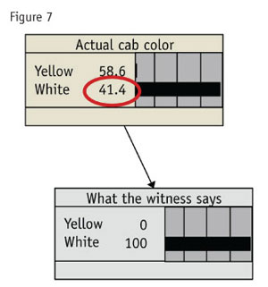
As we can see, the odds of the cab actually being white are about 41.4 percent, given that 85 percent of cabs are yellow and the witness is 80 percent right in identifying colors.
We have just come upon something difficult about Bayes nets. We have neatly and simply solved a problem that would have eluded most of us. And yet the correct answer seems strange. This is a difficulty we have with conditional probability. As Yudkowsky3 aptly puts it: “Bayesian reasoning is very counterintuitive.”
In sum, we have an approach that is powerful and hard to work out in our heads.
The three-door Monty Hall problem
This is a classic that has generated numerous arguments among scientists, statisticians, random onlookers and fans/foes of Parade magazine puzzle columnist Marilyn vos Savant. Here’s the problem:
There is a prize behind one of three doors. You pick a door. The sneaky game host does not tell you whether your door has won. Instead, he opens another door where there is NO prize. Then he asks whether you would rather switch doors OR stay with your door.
What do you do?
A statistician has shown on the Web how he nearly got this right by setting up 10,000 simulation runs in SPSS4. We will solve it with a simple three-node network.
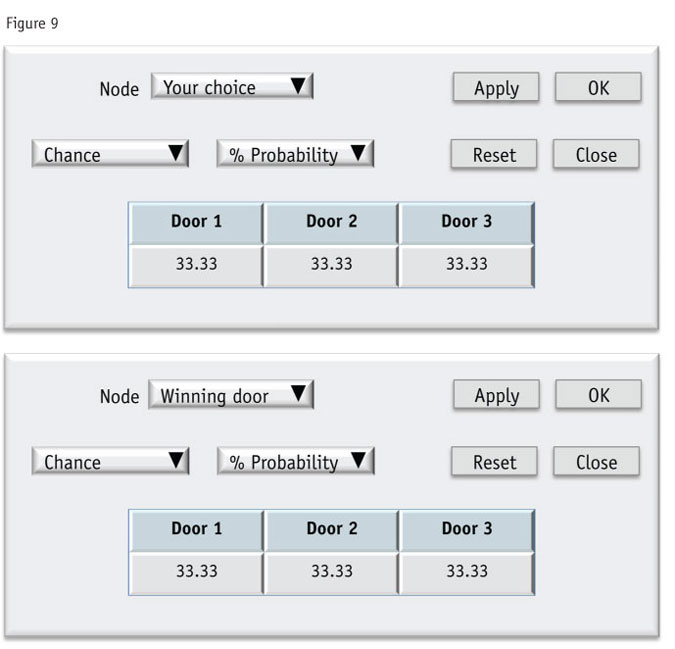
Setting up is critical. First we have two independent events (Figure 8): the door you pick and the door that wins. However, the door that is opened depends on both your choice and the winner.
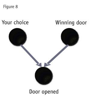
So these two independent events are now linked by the event of the door being opened (it depends on both of them). Each of the independent events has a probability of 33 percent for each door. This part is very straightforward (Figure 9).
Now on to the key: which door gets opened, based on which one you have chosen. This is going to take some thinking and, echoing Mr. Yudkowsky above, this part is not completely intuitive.
We have made a table (Figure 10) showing what happens with your choice and which door wins. Here goes. The table starts by saying you could choose Door 1, Door 2 or Door 3. For each of your choices, the winner could be any of the doors. So we have Doors 1, 2 and 3 within each of the three doors as the headers for the rows.

Now we have to cross these rows with which door gets opened. So at the top of the table, the column headers are “Opens 1,” “Opens 2” and “Opens 3.” We now start to see some surprising relationships.
Right away we can see that the odds of any door getting opened do not match. Just looking at this table, it seems lopsided – not what we would expect if the chances are even. A table with even chances would look completely symmetrical.
Anyhow, the (perhaps not) surprising answer to the three-door problem: You should switch!
The diagram in Figure 11 may take a little explaining but it shows the result. In it, we have moved your choice to “Door 1.” Now Door 1 cannot be the one opened so the sneaky host opens Door 2. The bar in “Door opened” gets moved to reflect that. “Your choice” and “Door opened” have taken on a grayish color to show that they are being changed.
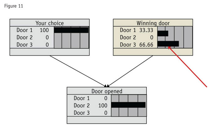
Not only should you switch but the odds favor you switching by 2:1 (66.6 percent for Door 1 vs. 33.3 percent for staying with your door). The red arrow points to the door with the best odds of having the prize – namely, the other door.
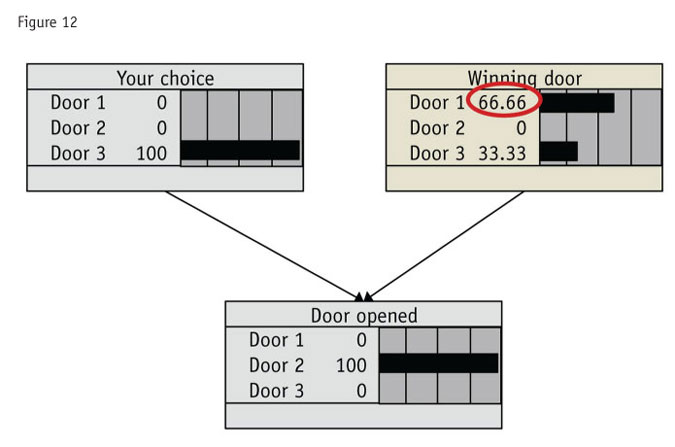
Now just to confirm that this is not a fluke, we change the doors (Figure 12). Now you choose Door 3 and the host opens Door 2. Once again, the odds favor a switch: 66.6 percent to 33.3 percent for staying.
If this seems confusing, if not impossible, you are in good company. About 10,000 people wrote to Marilyn vos Savant when she published the correct answer saying she was wrong. About 1,000 of those people had doctorates.
As we said above, the conditional logic used in networks is extremely powerful but not always intuitive, even if it gets the correct answer quickly.
To review, what tends to trick us is that the actions of the host have caused a link between two events that are otherwise independent. Now we see two points: these events are connected and the choice the host makes connects them. We then can understand how change will flow through when one of the events changes.
From the perspective of looking at a network, changes in probability must propagate (flow) through the network regardless of the way the arrows point.
May pose problems
Networks can use standard statistical tests to determine structure but these tests may pose problems. In fact, many problems related to networks are called “hard” in statistical language. Sometimes you will see the term “NP-hard” (which also may describe the reading that follows). Practically speaking, NP-hard problems can be insoluble – and that definitely would slow down your work.
In a network, if we rely on tests of significance, it is often difficult to choose the appropriate tests and good thresholds for those tests, because relationships can be numerous and highly complex. We also might be forced to reduce the number of statistical tests or reduce the number of variables processed, in an attempt to increase the tests’ reliability.
Networks gain more power if they use “value of information” as a basis for understanding structure. Information has value inversely proportional to its probability. That is, describing high-probability events has low information. Alternatively, high levels of information consist of describing low-probability events accurately.
This is not statistics as we have known it. Rather, testing balances the value of information vs. the length of description in machine language.
As you read about networks, you will encounter the minimum description length (MDL) principle. It is based on the idea that any regularity in a data set can be used to compress the data – to describe it “using fewer symbols than needed to describe the data literally.”5
Therefore, the best explanation is the one that minimizes description length while conveying the most information. As a general practice, information theory has sought to keep the cost of describing the data equal to or less than the value of the information in the data.
This is an excellent idea with very large data sets. There is plenty of data and it makes sense to balance how much information we gain precisely against how much effort it takes to describe that information. Using survey data and typical sample sizes though, we may need to explore different ratios of description vs. information to see patterns clearly.
May seem puzzling
Regressions are equivalent to a “naïve Bayesian” network. In a naïve Bayesian network all the variance in the target variable is portioned out to the dependent variables. And indeed, this is just what happens in a regression. This may seem puzzling (is this becoming a refrain?) but one way to describe the independent variables in a regression is as explaining the dependent. That is, each independent variable accounts for some of the variance or pattern in the dependent variable.
We have become accustomed to talking about the independent variables as predicting or driving the independent. However, if we think of the coefficients in a regression, we can see that each independent variable actually makes up some part of the total value of the dependent variable. We sum up the contribution of each variable times its coefficient and that total is the predicted value of the dependent.
Bayes nets of course differ from regression in important ways. Regressions are supposed to use continuous dependent variables (or with logistic regression, binary ones). Bayes nets were developed for use with discrete (categorical) variables. Many programs that create and analyze networks still only can handle variables of this type.
However, in recent years, networks have been extended and now can analyze continuous variables as well. The math involved is very abstruse indeed – but it works.
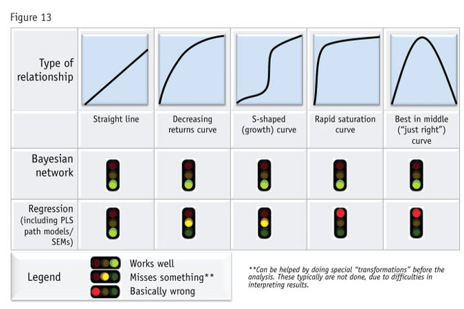
Regressions are supposed to have straight-line relationships among variables. This means all relationships, not only between the dependent and the independents but among all the independent variables as well. Bayes nets can handle any regular relationship between variables, whether it is linear or not. Figure 13 shows where each method is relatively likely to find success.
Find logical patterns
Next month we will return with two remarkable examples of the practical uses of Bayes nets, showing how they find logical patterns even in messy data, and then giving an example of how they linked survey questions to market share with remarkable predictive activity. In short, we will see two demonstrations that show just how these nets may be the “best newest thing” in understanding data. Stay tuned.
References
1 Stanners, W. (1999). “Essay on Bayes,” Game Theory and Information.
2 Thanks to Lionel Jouffe for this example.
3http://yudkowsky.net/rational/bayes
4http://www.uvm.edu/~dhowell/StatPages/More_Stuff/ThreeDoor.html
5 Perhaps the definitive work on this is Grünwald, P. (2007) The Minimum Description Length Principle (Cambridge, Mass.: MIT Press). That’s all we can say about it in this article.