
Editor's note: Keith Chrzan is senior vice president of analytics at Sawtooth Software Inc. He can be reached at keith@sawtoothsoftware.com.
Random forest (RF) analysis is pretty much the Swiss Army knife of quantitative methods. I’ve used it more and more over the years, so I thought it might be valuable to show how marketing researchers can use it through the brief case studies below.
What is a random forest? RF is a machine learning method based on, as the name suggests, a collection of trees – in this case a collection of decision trees. A decision tree is a way of segmenting a set of observations so as to create highly differentiated subgroups.
For example, the first decision tree I worked on was to help commercialize satellite TV. I’ve disguised this example a little, even though it was over 35 years ago. After describing the concept to respondents, we asked them how likely they would be to buy satellite TV and how much they would pay for programming.
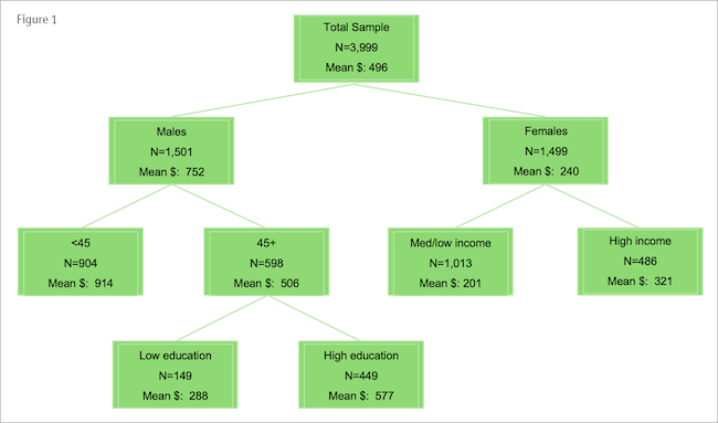
The decision tree analysis works by making a sequence of splits of respondents. In our TV case, first it went through all the variables in the survey to find the single one that best split our sample of respondents into higher- and lower-spend groups; this turned out to be whether the respondent was male or female. Then, among the male respondents the analysis searched all the variables and found the one (age) that best split the males into higher- and lower-spend groups. It also looked to find the variable (in this case, income) that best split female respondents into a group of lower spenders and a group of higher spenders. The tree continued splitting the subgroups (older male, younger male, higher-income female, lower-income female) branching more and more, until hitting some stopping rules (e.g., the groups or the differences between them get to small). The tree looked something like the one shown in Figure 1.
A decision tree can predict pretty well but it turns out that having a bunch of trees can predict even better than having just one. That’s where the “forest” part of RF comes in. The “random” part happens because we generate each tree using two varieties of randomness.
First, for a given tree the analysis selects a bootstrap sample of the same size as the original sample (by default, but users can adjust this). Because we draw this sample with replacement, this leaves little over a third (about 37%) of the original sample out of a given tree (the analysis then cleverly uses this holdout sample for validation).
Next, at each branching step, the analysis considers only a subset of the available variables. How big a subset is something we decide upon when setting up the forest. By default the analysis includes one-third of the variables or the square root of the number of variables, depending on whether the forest predicts a metric or a categorical variable, respectively.
So, if the satellite TV study had 3,000 respondents, the first tree would include about 1,900 of them (some more than once, for a total of 3,000) and leave as holdout sample about 1,100 of them. The first branch of that tree might include only 20 of the original 60 predictor variables, while the next branch would include a different 20 predictor variables. And so on for each of the 500 or 1,000 trees we program into our forest. Each tree has a different bootstrap sample of respondents and at each branch of each tree we consider a new random draw of the possible predictor variables. The two randomizing steps are said to “de-correlate the tree,” meaning that the forest is less subject to the ill effects of collinearity than any single tree would be.
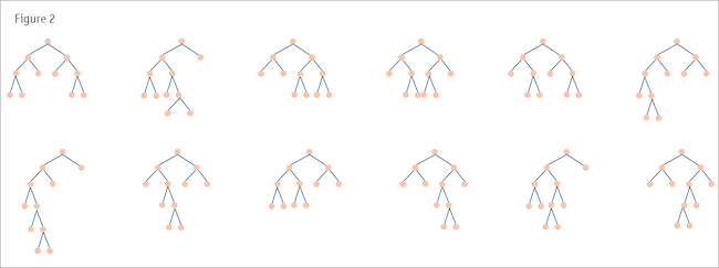
What we end up with is a forest of these purposely impoverished trees, say like the subset of 12 trees from a larger forest shown in Figure 2.
If it’s a categorical variable we’re predicting, each imperfect tree gets a vote and we simply count votes to make our prediction. If it’s a metric variable, we just average the prediction across trees to come up with the forest’s prediction.
Six common uses of RF
With that brief introduction behind us, let’s look at some ways marketing researchers can use RF analysis.
1. Driver analysis with mixed or categorical variables
My first experience with RF came when I needed to run driver analysis and I had a mix of metric and categorial predictors. Driver analysis often features correlated predictors (i.e., it suffers from collinearity) which can produce misleading results when we use traditional methods like correlation and regression analysis. Newer methods (averaging over orderings, Johnson’s relative weights) largely resolve the collinearity problem for models with metric predictors like ratings, counts and percents. When you have any categorical predictors in the mix, however, those methods struggle. RF doesn’t. As noted above, the two randomization steps involved in RF (different subsets of respondents per tree, different subsets of variables considered at each split in each tree) decorrelate the forest and allow it to overcome collinearity. Moreover, unlike the other driver analysis methods, RF is agnostic about whether variables are metric or categorical.
In a concept test a client wanted to know which factors (a mix of attitudes, behavioral counts and percentages and categorical demographics) most inclined survey respondents to report interest in a new product. The RF analysis was able to overcome both the collinearity in the data (there was plenty, especially in the ratings) and the fact that we had a mix of metric and categorical predictors. The RF model produced a set of relative importances, one per predictor. We typically rescale these to sum to 100 for convenient interpretation. The RF could also have produced a predictive model for my client, but the client’s interest was only on understanding the drivers, not on using them to predict.
2. Driver analysis with a multi-category dependent variable
It turns out that RF is also agnostic about the scaling of the dependent variable in a driver analysis model.
In a patient chart study, my client collected data from the medical records of three patients from each of 300 physicians, for 900 patients overall. The client wanted to use facts about the physician, the patient, the patient’s disease state and history (some 40 variables in all) to predict which of four therapies the physician would recommend. The RF model quantified the relative importance of the variables. Not surprisingly the patient and particularly the disease-state variables turned out to be the most important, much more important than variables describing the physicians.
3. Variable selection for predictive segmentation
The next two uses for the importances that come out of RF involve variable selection for segmentation studies. Variable selection is a crucial, and often overlooked, step in segmentation. Doing it properly solves a complex of problems that plague the segmentation studies produced by inexperienced analysts: the problem caused by masking variables that hide rather than reveal the structure in the data and the (rightfully) spooky-sounding problem named the curse of dimensionality (the curse causes segments to be more similar and less distinct as the number of variables gets larger).
In segmentations where we want the segments to differ with respect to one variable (usually purchase intent for a new product) we like to do predictive segmentation where we include as basis variables for our segmentation analysis only such variables as are correlated with the variable of particular interest.
In a recent segmentation study, we wanted the segments to differ in terms of their level of interest in a new line extension for a successful older product. In addition to purchase intent and other standard concept testing metrics we also collected respondent demographics, their category-specific attitudes and their ratings of some general lifestyle attributes. Using RF, we identified a subset of these (a demographic, five category-specific attitudes and four general lifestyle attitudes) that were highly correlated with the purchase intent. When we used those 10 variables in a latent class cluster analysis (because the demographic variable was an unordered categorical variable, latent class made more sense than distance-based clustering) we found four segments of respondents with very different levels of interest in the line extension. The segments also differed in terms of the 10 basis variables, which gave the marketing team the levers they needed to pull to market differently to the resulting segments.
4. Variable selection for unsupervised segmentation
More often, however, we don’t have a one variable of particular interest. In this case we use something called an unsupervised RF. The name may sound like an oxymoron, but it turns out the method isn’t really unsupervised at all. First, the analysis makes a copy of the original data set except that it randomly and independently sorts each column of variables. This breaks all relationships in the copied data set. It then labels each record from the original set “1” and each from the copied/broken data set “2.” The program then uses this as a dependent variable and runs an RF to distinguish whether a record comes from the original data set or the copied/broken data set. This unsupervised RF analysis quantifies the relationship of each potential segmentation basis variable with the segmentation structure present in the data. By selecting only the most important variables revealed by the RF, the analyst avoids masking variables and the curse of dimensionality at the same time.
A client was considering almost twice as many basis variables as they had respondents in a segmentation study, which they realized was pretty much a red-carpet invitation to the curse of dimensionality. Using an unsupervised RF, we culled the list of 250+ potential basis variables down to a manageable set of around 15. Since there were many possible subsets of variables to choose from the longer list (1.8 x 1075 such subsets, actually) having an organized approach for choosing the best subset prevented a lot of going back and forth trying different subsets of variables, keeping the segmentation study on track and on budget.
5. Creating a similarity matrix as the basis for a segmentation
It turns out that the unconditional RF also produces a similarity matrix of the variables. When you have a mix of metric and categorical basis variables for your segmentation, creating this RF similarity matrix is one way of accommodating the mix of variable types (other methods for handling mixed variable types include latent class models).
Recently a client wanted to segment their market using survey data. Variable selection analyses identified a mix of metric and categorical variables as viable bases for the segmentation. The client requested that we investigate a broad range of potential solutions before deciding which to share with their stakeholders. A latent class segmentation resulted in viable-looking three-, four- and five-segment solutions. We also ran the unsupervised RF and input its proximity matrix to a k-medians cluster analysis program, which gave us viable three-to-six-segment solutions. In the end the client went with the four-segment latent class solution, but as they had specifically requested we come at the analysis from multiple angles, the RF/k-medoids approach helped us out quite a bit.
6. Typing tool creation
Once we’ve created our segments, we can use RF to build a classification model. RF classifiers tend to be very parsimonious, but instead of producing simple typing equations they need to have new survey data run through the forest, which can limit their applicability (alternatively we can sometimes create a lookup table of every possible combination of inputs and use that for on-the-fly typing).
For example, in a segmentation study we did a few months back, we found that classic typing tools (discriminant analysis, multinomial logit) performed less well than the client wanted: with seven variables we could classify respondents into five segments with 63% accuracy, which rose to 68% if we used 12 predictors. However, with just five variables, an RF classifier had 80% accuracy and with 12 that accuracy topped 95%. The five-variable RF typing tool needed a 16,807-row lookup table (feasible in Excel) while the 12-variable tool required a 13.8 billion-row table, which of course was not so practical.
6a. Building an armada of space robots to defend the Earth from alien invasion
Actually, just kidding about this one – the code for this RF model isn’t fully debugged yet.