Editor's note: Michael Lieberman is founder and president of Multivariate Solutions, a New York-based consulting firm. He can be reached at michael@mvsolution.com.
The definition of game theory has been changing recently. ESPN has co-opted it to describe basketball statistics, chances of a winning hand the Poker World Series or e-sports leagues.
Of course, words change meaning all the time. For example, before World War II a brainstorm meant a violent outburst. Today, as a verb, it is a process of trying to “solve a problem or come up with new ideas by having a discussion that includes all members of a group” (Merriam-Webster) – in other words, a good vehicle for ordering a full menu of appetizers at 6:00 p.m.
Game theory, in its true form, is the discipline that studies how agents make strategic decisions. It was initially developed in economics to understand a large collection of economic behaviors, including firms, markets and consumers. Later on, we may find game theory in social network formation, behavioral economics, ethical behavior, biology, political coalition forming and bargaining decision theory. Game theory is applied in continuous loops in modern machine learning algorithms to model consumer choice.
In this article, I will cover the basics of game theory. Along the way, I will touch on some of the words bandied about in the marketing research industry, such as Nash equilibrium, Bayesian statistics and the Shapley value. I will explain the fundamental differences between the two game theory models. Finally, I will share a case study to show how progress in highly sophisticated, open-source software has noncooperative game models well within the marketing research quiver.
Modern game theory begins with the publication of John von Neumann and Oskar Morgenstern’s book, “Theory of Games and Economic Behavior,” which considers cooperative games with several players. The emergence of game theory led to the popularization of the Nash equilibrium and Shapley value regressions. I took a course in game theory in 1986 as a senior majoring in mathematics at Rutgers University. It was mathematically challenging, given that we were calculating pre-personal computer complex algorithms that, when transformed by logit regression, became the chances of a decision being made, a Bayesian interpretation of probability where probability expresses a degree of belief in an event – the simple definition of Bayesian statistics.
Cooperative games
There are, essentially, two types of game theory models. The first is a cooperative game: a coalitional game with transferable utility, involving a set of players, is a cooperative game that can be described as a function that associates a real number with each group, which is the worth of the coalition. If a coalition forms, then it can divide its worth in any possible way among its members. Thus, each player is trying to figure out how much is the maximum they can get while keeping the coalition intact.
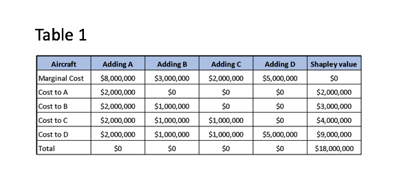
If there are four airlines and we run a cooperative game to see how much they should each pay for, say, an airfield based on airline usage, the amount calculated by the software for each player is the Shapley value. The Shapley value of each player is a unique contribution of total costs borne by each player.
This would be the R stat code:
> BUILDINGCOST <- c(8000,11000,13000,18000)
> AIRLINES <- c("Airline A","Airline B","Airline C","Airline D")

Noncooperative games – consumer/brand behavior
The second type of game is called a noncooperative game. In noncooperative game theory, a game is a detailed model of all the moves available to the players. A noncooperative game is a game with competition between individual players, as opposed to cooperative games, and in which alliances can only operate if self-enforced. The key distinguishing feature is the absence of external authority to establish rules enforcing cooperative behavior (e.g., court system). In the absence of external authority, players cannot group into coalitions and must compete independently. The maximum point at which each player is satisfied and no player can gain more without angering the other players is called the Nash equilibrium.
A good example of cooperation in a noncooperative game is the Hasbro board game Risk. Essentially every player is out to win – by definition a noncooperative game. However, if there are five players, and four players want one player out. They form a coalition (cooperative game) and beat the player down (defining the temporary rules of a noncooperative game). Once that player is gone, they turn on each other.
This might sound familiar because it happens almost daily in the real world. A crowded primary political race. Corporate takeover alliances among shareholders with different agendas but a common enemy. Brand competition to increase market share when there might be a dominant player.
What if?
Legally brands are not allowed to cooperate like the players in our Risk example. This can be labeled as price-fixing or monopolistic behavior. Thus, most branding teams rely on consumer-focus strategies for pricing, advertising and brand marketing.
Several brands within a finite brand space are in constant competition for market share. A common study to determine optimal pricing is choice-based conjoint analysis – also known as a discrete choice model. A well-formed discrete choice model will yield a relative pricing coefficient for each brand in the study (computed with a logistic regression for choice). It will also yield a choice coefficient, which is brand preference within the study. Together these two coefficients can estimate market share within the frame of the study. They are input into a marketing model for the savvy marketing researcher.
In the constant back-and-forth of brand wars, real-world applications of marketing mix models are unceasing. Empirical research shows that brand managers tend to react to their competitors’ marketing moves more than they may need to. This is a shift in marketing strategy from customer-focused to competitor-focused strategy.
Quite frankly, it makes sense. Coke just aired a new campaign. Is Pepsi not going to react? Managers may react over-aggressively. Many believe that marketing or pricing strategies of their competitors’ may have more effect than they actually do, particularly in relatively stable product categories.
There is an assumption in a brand space that it is in equilibrium. Brands are not allowed to collude, but brand cooperation is a regular practice – like the four players in the Risk example above. The big players kind of figure out how much a product should cost. They analyze their competitors’ marketing and digital strategies. They make assumptions, meaning that their information is not complete (they may not have a competitors’ advertising budget). It is natural to conclude that brand managers will do what’s best for their brand. What if they conclude that imitating a competitor’s marketing or pricing moves might actually be in their brand-share interest?
When a brand in competition space makes a move, it is assumed that the market then is in disequilibrium. That is, a competing brand manager must do something to react to protect their market share. This is usually the case. But what to do is where the utility of game theory of noncooperative games comes in. What if a new competitor enters the market? A new product? A disrupter? What is the strategy?
The expansion of computing power
Because running noncooperative games in R stat is very easy, running multiple scenarios is like running perpetual marketing mix models simultaneously. The goal is to estimate how the players’ utility for each possible outcome varies as a function of observed variables, like annual sales, known market share, price, advertising budget, etc. Many of these inputs may come from survey data or secondary data. It is a dynamic output, meant to give clients data for data-driven decisions – the outputs of a discrete choice model mentioned above.
For example, a competitor lowers their price for a promotion. What should the marketing strategy be?
An illustrative advertising game
- Two firms (A and B) must decide how much to spend on advertising.
- Each firm may adopt either a higher (H) budget or a low (L) budget.
Firm A makes the first move by choosing either H or L at the first decision “node.” Next, B chooses either H or L, but the large oval surrounding B’s two decision nodes indicates that B does not know what choice A made (Figure 1).
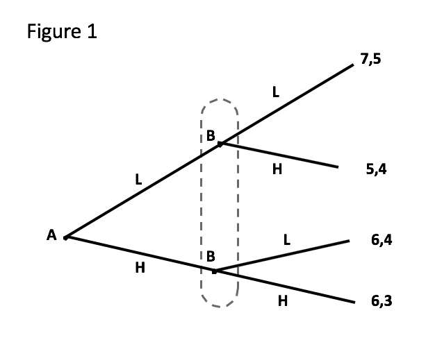
The numbers at the end of each branch, measured in thousands or millions of dollars, are the payoffs. For example, if A chooses H and B chooses L, profits will be 6 for firm A and 4 for firm B.
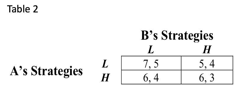
The game in normal (tabular) form is shown in Table 2, where A’s strategies are the rows and B’s strategies are the columns.
This is one scenario among thousands within this brand space. The perpetual game and payoffs can be written by machine learning algorithms that decipher the game and supply the client with unending data for data-driven decisions.
The applications of game theory to machine learning, marketing research lie at the intersection of statistical application and strategic reasoning. As technology advances, this will only become more common.