
Editor's note: Keith Chrzan is senior vice president of analytics at Sawtooth Software Inc.
Situational choice experiments (SCE) resemble the more commonly used choice-based conjoint experiments except they have different experimental design requirements and they ask for different cognitive operations on the part of survey respondents – both of which lead to a statistical model that differs from the conditional multinomial logit typically used in conjoint experiments.
First of all in this article, we’ll do a brief review of choice models and choice experiments. Then we’ll cover the steps in a situational choice experiment, from design to data formatting to analysis and reporting. The most common use case for SCE is modeling physicians’ therapy decisions. We also include two brief case studies showing other uses of SCE. A bit of background will clarify how SCEs differ from other kinds of choice experiments and from other kinds of choice models.
Choice models
The go-to analysis engine for choice modelers is the conditional multinomial logit (MNL) model (McFadden 1974, Ben-Akiva and Lerman 1985). Say we have a set of attributes that describe products (or services or, more generally, alternatives). And assume that alternatives differ from one another in terms of the specific levels they have for the attributes. We use conditional MNL to predict choice among alternatives based on the attributes and levels of those alternatives. For example, McFadden et al. (1977) interviewed commuters in San Francisco and predicted their travel choices (taking a bus, driving, etc.) based on attributes like travel times, wait times and costs. Guadagni and Little (1983) used scanner panel data from grocery stores to predict coffee purchases as a function of the brand, package size and prices of the products.
A special case of MNL is the polytomous multinomial logit (P-MNL) model (Theil 1969, Hoffman and Duncan 1988). With P-MNL, the attributes and levels do not vary across alternatives because they describe the chooser or the situation, not the alternatives. For example, the first time I used P-MNL was to predict the pregnancy decisions (terminate, give the baby up for adoption, keep the baby) of female prison inmates. P-MNL allows us to predict these choices as a function of facts about the woman’s sentence, the availability of parole and demographics like her age, education, family structure and so on.
Choice experiments
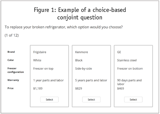
If we add experimental control in the design of stimuli, we have a choice experiment. The most familiar of these features multi-profile choice sets analyzed via conditional MNL, a combination known as choice-based conjoint (CBC), discrete choice experiments or stated choice experiments (Louviere and Woodworth 1983). In a choice-based conjoint experiment, we show each respondent a series of a dozen or so questions that look like the one shown in Figure 1.
An experimental design makes the attribute levels independent. This allows us to isolate and quantify the value of each level of each attribute, entities we call “utilities.”
This article concerns a less common type of experiment, a situational choice experiment. In a given SCE question, we have a single, experimentally designed profile that describes the situation or context of a decision and then two or more fixed alternatives from which the respondent can choose. In other words, the designed profile changes from question to question but the choice alternatives do not (hence, SCE uses P-MNL modeling). Across questions, the profiles conform to an experimental design. A single SCE question might look like the one shown in Figure 2 (note, this is a fictional example and these are not the therapies one would use to treat hepatic sarcoidosis).
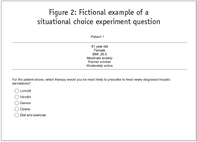
In the next several questions, the description of the patient changes but the five choice alternatives remain the same. So, the patient in the next question might be a 64-year-old inactive female smoker with a BMI of 23 and severe anxiety, for example. The only way for the alternatives’ probabilities to differ is to have a separate set of utilities for each of the five choice alternatives. The P-MNL does this. Whereas CBC produces a single vector of utilities, P-MNL gives us a matrix of utilities, one vector for each alternative.
To review, SCE differs from CBC experiments. CBC uses experimentally designed sets of two or more profiles and uses conditional MNL. An SCE, on the other hand, uses experimentally designed profiles, shown one at a time, and uses polytomous MNL. Both produce utilities that predict choices among alternatives.
Few marketers know about SCEs and there does not seem to be a single source reference about them, two limitations the author hopes to remedy in this article. The next section walks through the steps involved in conducting an SCE, including a discussion of sample size. The final section describes commercial marketing examples of SCEs.
Executing a situational choice experiment
Research design
Before choosing a design strategy, we need to know how many attributes and how many levels per attribute to accommodate. SCE sample size requirements increase with the number of attributes and levels. Most SCEs the author has run have had fewer than 10 attributes.
We construct an SCE design using an efficient design for single-profile experiments. Sawtooth Software’s Lighthouse Studio, SAS and the design program Ngene from ChoiceMetrics all have efficient design algorithms that fit the bill, regardless of the number of attributes or the number of levels per attribute. For the special case in which all the attributes have the same number of levels, traditional orthogonal experimental design plans also work (Addelman 1962). The experimental designers currently available in R also work in this case. In practice we usually use software that makes our design in several blocks. Each respondent receives a randomly assigned block of questions. Software allows the user to specify how many questions each block contains while the orthogonal design plans tend to come in set sizes, which may not be convenient or respondent-friendly.
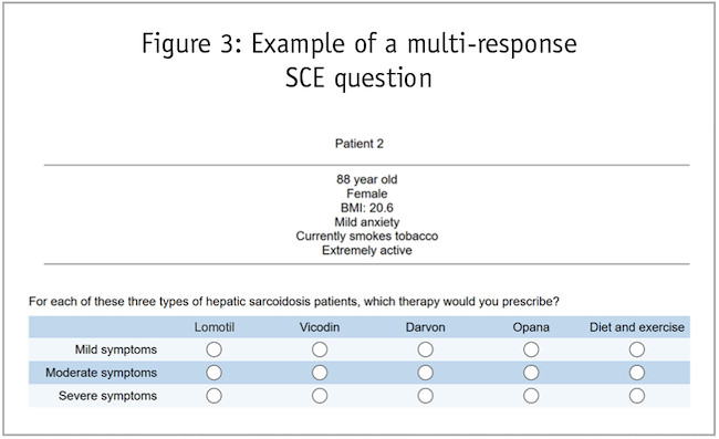
Design in hand, we net produce the SCE questionnaire, giving each respondent the questions from a given block in the experimental design. In addition to asking a single response as in the example above, we might ask for separate responses for different segments, as shown in Figure 3.
In some cases, we might want respondents to allocate their last 10 patients to treatments or to ask about the percentage of patients to which they would recommend each therapy (Figure 4).

Data structure
We next collect respondents’ choices for each question and add them to the experimental design matrix. Now we have our data file ready for analysis. For example, the hepatic sarcoidosis data from a single respondent might look like Table 1.
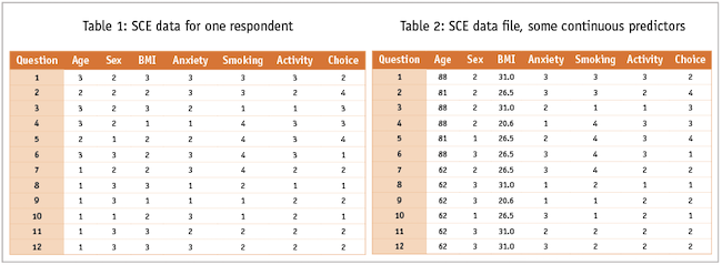
In the analysis software we might treat the predictors as categorical. Alternatively, we might to treat age and BMI as continuous variables. In this case, our data from the first respondent might look like this Table 2.
To create our analysis data file we simply concatenate the 12 rows of data we get from each respondent; in this example where each respondent makes choices for each of 12 patients, our analysis data file would contain 12 times as many rows as we have respondents.
Modeling and reporting
General-purpose statistical software like SAS, SPSS or SYSTAT offer canned P-MNL routines. You can also access such programs through specialty choice modeling packages like NLOGIT from Econometric Software, the mlogit and nnet packages in R or in the MBC program for logit modeling from Sawtooth Software. Because P-MNL is a special case of conditional logit, you can also trick conditional logit software into running P-MNL analysis. This can be handy when you collect constant sum data as in Figure 4.
Analysis will produce a set of model coefficients (utilities), one per level in the dependent variable. One column of all zeros represents the reference level of the dependent variable. For example, the utilities from our hepatic sarcoidosis example might look like those shown in Table 3.
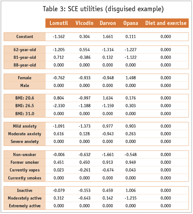
In this model, all predictors were categorical, so that each has a reference level row set to zero. Of course, the statistical software will also produce standard errors and model fit statistics. These allow us to calculate the p-value of each of our utilities and to test alternative models.
Some academic modelers prefer to express the results as “odds ratios.” To do this they exponentiate the utilities. With most marketing audiences, however, taking a number they do not understand, transforming it in a way they understand even less to produce numbers without an intuitive meaning to them is hardly a winning communication strategy.
Simulations
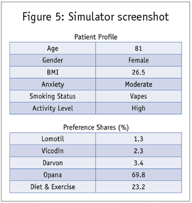
As a result, we typically deliver the model results to clients in Excel simulators. Using the same equation that calibrates the utilities from the choice response data in the first place, we can predict shares given any profile specified in terms of the attributes and levels. Thus, marketers need not even see the utilities. Simply using drop-down menus for each attribute, the user can create a profile and then get share estimates, as shown in Figure 5.
Sensitivity analysis showing how shares change as patient descriptors change can directly inform marketing decisions.
Other modeling options
Modelers usually prefer mixed logit (which produces a set of utilities for each individual respondent) for their CBC experiments. Because of how sparse the data matrix is for SCE, however, we see a diminished benefit of generating respondent-level utilities. Even with the diminished benefit, however, having respondent-level utility models comes in very handy when building simulators that allow users to look at results for subgroups of respondents.
Sample size
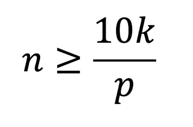
Peduzzi et al. (1996) recommend that sample size for a logit model should be at least 10 times the number of parameters in the model divided by the choice probability for an alternative:
where
n is the sample size
k is the number of non-zero parameters (utilities) to be estimated by the model
p is the probability of the least frequently chosen alternative
Imagine an SCE with six four-level attributes and five choice alternatives. The model will have a constant and 6 x 3 = 18 parameters per utility function. With four non-zero utility functions that totals 76 utilities. With five choice alternatives – and assuming we don’t know which alternative will be the least chosen – the average probability of choice is 20%, which suggests a number of observations of at least:
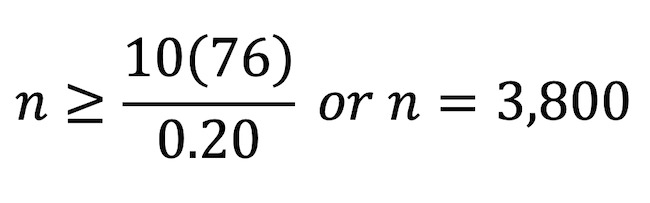
If we ask 10 SCE questions of 380 respondents, we can get our sample size target.
Another sample-size rule of thumb comes from thinking about the sampling error around simulation shares. We know that a sample size of 100 produces margins of error of 0.098 for percentages and that halving that margin of error requires quadrupling the sample size. The sample size of 380 above would produce shares with margins of error of 0.05. For small experiments, the simulator margin of error will drive sample size more than will the Peduzzi et al. rule of thumb, but the latter will have more influence as the number of attributes, levels and (especially) choice alternatives increases.
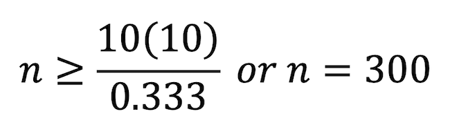
For example, an experiment with four two-level attributes and three choice alternatives would suggest a minimum of 300 observations:
Asking each of 30 respondents 10 SCE questions would get you the minimum number of observations from the Peduzzi et al. formula. Unfortunately the sampling error around shares for a sample of size 30 would be an excessive +/- 0.18, or 18 percentage points.
Case studies
Therapy choice experiments
The patient-type experiments such as the hepatic sarcoidosis example above are the most common application of SCE. These have small numbers of attributes, typically four to eight, and also small sample sizes. The populations from which we draw physician respondents come are small and they expect expensive honoraria for their participation in survey research.
Durable acquisition decision
In a study of high-priced industrial durables, a client wanted to know what product profiles drive preference among brands. CBC could answer that very nicely. But the client also wanted to know whether the industrial customers would opt to lease or to buy the products they chose. For this, we created a CBC experiment in which respondents faced a choice among three experimentally designed product profiles. After choosing the profile they most preferred, respondents answered an SCE question about that most preferred profile: Given what they know about the market, the products and prices available and their budgets, would they buy the product they selected, lease the product they selected or neither buy nor lease the product?
We combined both models into an Excel-based simulator and the client was able to see, for any product specified and in any competitive set, how many respondents preferred it more than the other products and how many of those would lease the product, buy it or go without it.
Retirement hybrid experiment
A financial services company wanted to forecast how many of its savers who would choose to retire and start drawing down their retirement accounts. An SCE featured attributes and levels that described the economic conditions (interest rates on investments, growth in home prices, inflation, recent and forecasted economic growth). We also had information on the savers stored in a database: their age, amount of savings, income, credit histories and so on. This additional information didn’t conform to an experimental design but we included it in the model anyway – it would be silly to ask a 64-year-old married man with $750,000 in retirement savings answer our questions as if he were a 58-year-old single woman with $1,200,000 in the bank. We had experimental control over the variables we designed into the SCE but we also had the database variables to provide even more context to the respondents’ reactions to the SCE questions.
Increases awareness
Hopefully this introduction to situational choice experiments increases awareness of this little-known cousin of conjoint analysis. If so, it will help add a powerful new methodology to the researcher’s toolkit.
References
Addelman, S. (1962). “Orthogonal main-effect plans for asymmetrical factorial experiments.” Technometrics 4(1): 21-46.
Ben-Akiva, M., and Lerman, S.R. (1985). “Discrete Choice Analysis: Theory and Application to Travel Demand.” Cambridge, Mass.: MIT Press.
Guadagni, P.M.. and Little, J.D.C. (1983). “A logit model of brand choice calibrated on scanner data.” Marketing Science 2(3): 203-238.
Hahn, G., and Shapiro, S. (1966). “A catalogue and computer program for the design and analysis of orthogonal symmetric and asymmetric fractional factorial designs.” Report for Research Development Center. Report no. 66-C-165. Schenectady, N.Y.: General Electric Corporation.
Hoffman, S.D., and Duncan, G.J. (1988). “Multinomial and conditional logit discrete-choice models in demography.” Demography 25: 415-427.
Louviere, J.J., and Woodworth, G.G. (1983). “Design and analysis of simulated consumer choice or allocation experiments: an approach based on aggregate data.” Journal of Marketing Research 20: 350-367.
McFadden, D. (1974). “Conditional logit analysis of qualitative choice behavior.” In: P. Zarembka (ed.) “Frontiers in Econometrics.” New York: Academic Press, pp. 105-142.
McFadden, D., Talvitie, A., and associates (1977). Report for Urban Travel Demand Forecasting Project, Phase 1 Final Report Series, Volume V. Report no. UCB-ITS-SR-77-9. Berkeley: University of California.
McFadden, D. (2001). “Economic choices.” American Economic Review 91(3): 351-378.
Peduzzi, P., Concato, J., Kemper, E., Holford, T.R., and Feinstein, A.R. (1996). “A simulation study of the number of events per variable in logistic regression analysis.” Journal of Clinical Epidemiology 49(12): 1373-1379.
Theil, H. (1969). “A multinomial extension of the linear logit model.” International Economic Review, 10(3): 251-259.